Satellite Image Processing with Deep Learning¶

20 Aug 2026

Info

This notebook was created for a workshop held at ADA University (17–21 August 2026).

Tip

Run this notebook in Colab for the easiest setup (GPU is optional, large downloads may take time).

Satellite imagery is different from the images we usually encounter in computer vision. A satellite can measure wavelengths that humans cannot see, repeatedly observe the same location over time, associate every pixel with a geographic location, and even use radar to observe the Earth's surface through clouds and other atmospheric effects. Just like other domains, such distinctive properties change how we apply deep learning to satellite imagery. In this notebook, we will work with real satellite data, visualize different spectral bands, process GeoTIFF files, construct multispectral images, prepare satellite data for neural networks, and examine some of the problems that make deep learning for satellite imagery different from conventional computer vision.

Optical vs Radar Satellite Imagery¶

Satellite sensors can observe the Earth in different ways. Two particularly important types of satellite imagery are optical imagery and radar imagery.

Optical satellites measure electromagnetic radiation reflected from the Earth's surface. This includes visible light, but satellite sensors can also measure wavelengths outside the range visible to humans, such as near-infrared and short-wave infrared. These additional measurements allow us to distinguish properties of vegetation, water, soil, snow, built-up areas, and other surfaces that may not be obvious from RGB images alone. However, optical imaging depends on the radiation reaching the surface and then reaching the satellite sensor. Clouds and other atmospheric effect can therefore obscure the Earth's surface in optical images, and ordinary passive optical imaging also depends on illumination.

By User:Zedh and User:Gringer, CC BY-SA 3.0, Wikimedia Commons.

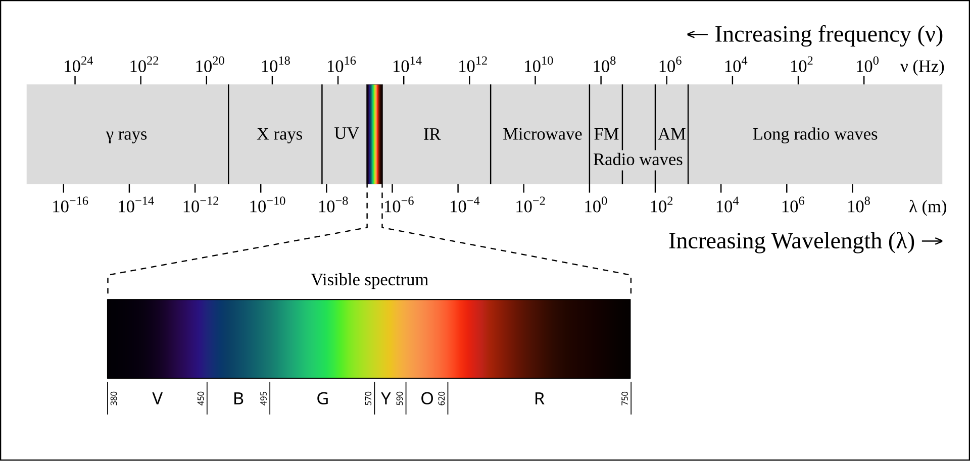
Radar satellites are active sensors: the satellite transmits microwave signals toward the Earth and measures the signal returned to the sensor. Because radar uses longer wavelengths than visible and infrared light, it can operate both during the day and at night and can observe the surface through most cloud cover. Synthetic aperture radar (SAR) is the most commonly used imaging radar technology in Earth Observation (EO).

Satellite Missions¶

Different satellite missions are designed for different types of Earth observation.

Sentinel-2 is an optical Earth observation mission. Its satellites carry multispectral sensors that measure reflected radiation in 13 spectral bands, covering visible, near-infrared (NIR), and short-wave infrared (SWIR), and other wavelengths. The bands are provided at different spatial resolutions: $10$, $20$, and $60$ m. This means that, depending on the band, one pixel corresponds to approximately a $10 \times 10$, $20 \times 20$, or $60 \times 60$ m area on the Earth's surface. Sentinel-2 is widely used for tasks such as vegetation monitoring, land-cover mapping, agriculture, water analysis, disaster assessment, and change detection. We will use Sentinel-2 imagery extensively throughout this notebook.

Sentinel-1 is a radar Earth observation mission based on synthetic aperture radar (SAR). Unlike Sentinel-2, it does not rely on reflected sunlight and actively transmits microwave signals and measures the returned signal (recall the previous section). Sentinel-1 can therefore acquire observations during both day and night and under most weather conditions. Its radar measurements are particularly useful for applications such as flood mapping, surface deformation, sea-ice monitoring, land-cover analysis, and situations where optical imagery is frequently obscured by clouds (e.g. cloud removal).

Landsat satellites provide multispectral optical and thermal observations of the Earth's surface. Landsat imagery generally has lower spatial resolution than the highest-resolution Sentinel-2 bands, but its long historical archive makes it particularly useful for studying changes over long periods of time.

The Sentinel missions are part of the European Copernicus Earth observation programme and are operated by the European Space Agency (ESA) together with European partner organizations. Sentinel-1 and Sentinel-2 have been providing observations since the mid-2010s. Landsat is considerably older: the programme began in 1972 and is jointly managed by the National Aeronautics and Space Administration (NASA) and the United States Geological Survey (USGS).

These missions are especially common in research, as their data are openly available, provide global coverage, and have large archives containing repeated observations of the same locations. They are therefore well suited for machine learning, where we often need large amounts of consistently acquired data. Sentinel-2 is particularly useful for multispectral deep learning because of its relatively high spatial resolution and 13 spectral bands, while Sentinel-1 provides complementary radar information.

These are not the only important Earth observation missions. MODIS, carried on NASA's Terra and Aqua satellites, provides much coarser spatial resolution but very frequent observations and has been widely used for large-scale environmental and climate monitoring. Commercial systems such as SPOT), PlanetScope, and WorldView can provide higher spatial resolution, sometimes down to a few metres or below one metre, but their imagery is generally not as freely available as Sentinel or Landsat data. Other missions are designed for more specialized measurements, such as precipitation, atmospheric composition, elevation, ocean properties, or hyperspectral imaging.

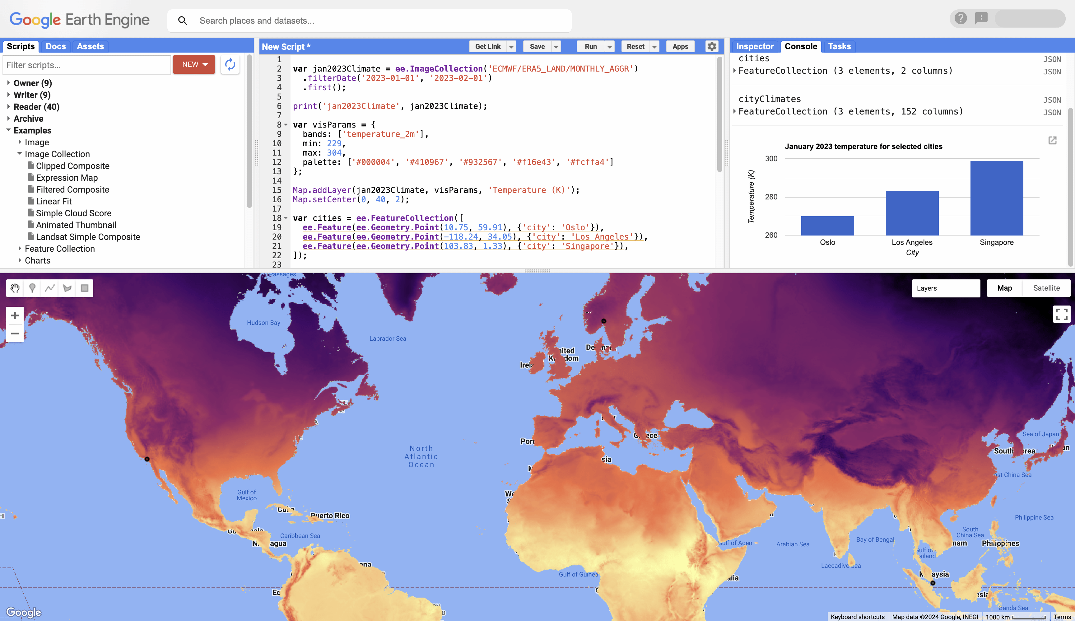
Satellite images can be obtain from their corresponding platforms. Cloud-based platforms such as Google Earth Engine (GEE) provide access to large satellite archives without requiring users to manually download entire collections. In machine learning, datasets derived from these missions are often distributed through repositories or libraries such as TorchGeo, which we will use in this notebook.

The Earth Engine Code Editor at code.earthengine.google.com. Retrieved from GEE get started manual.

For the practical examples in this notebook, we will primarily use Sentinel-2 data and later introduce Sentinel-1. Most of the concepts we develop, including spectral bands, spatial resolution, GeoTIFF files, preprocessing, patch extraction, and deep learning pipelines, also transfer directly to Landsat and many other satellite missions.

TorchGeo EuroSAT Dataset¶

Working directly with raw satellite products can require substantial preprocessing. Depending on the mission, a single observation may contain multiple files corresponding to different spectral bands, spatial resolutions, metadata, cloud masks, and acquisition information. For this notebook, we will initially use TorchGeo, a PyTorch library designed for geospatial machine learning. TorchGeo provides dataset classes, sampling utilities, transformations, and other tools that make it easier to work with common remote-sensing datasets while remaining compatible with the standard PyTorch workflow.

We will begin with EuroSAT, a land-use and land-cover (LULC) classification dataset derived from Sentinel-2 imagery. The multispectral version contains all 13 Sentinel-2 spectral bands and includes images from 10 LULC classes.

In [1]:

!pip install torchgeo==0.10.0 -q

!pip install torchgeo==0.10.0 -q

     ━━━━━━━━━━━━━━━━━━━━━━━━━━━━━━━━━━━━━━━━ 44.7/44.7 kB 2.8 MB/s eta 0:00:00
     ━━━━━━━━━━━━━━━━━━━━━━━━━━━━━━━━━━━━━━━━ 44.8/44.8 kB 2.9 MB/s eta 0:00:00
   ━━━━━━━━━━━━━━━━━━━━━━━━━━━━━━━━━━━━━━━━ 811.4/811.4 kB 26.5 MB/s eta 0:00:00
   ━━━━━━━━━━━━━━━━━━━━━━━━━━━━━━━━━━━━━━━━ 158.0/158.0 kB 9.8 MB/s eta 0:00:00
   ━━━━━━━━━━━━━━━━━━━━━━━━━━━━━━━━━━━━━━━━ 1.2/1.2 MB 35.5 MB/s eta 0:00:00
   ━━━━━━━━━━━━━━━━━━━━━━━━━━━━━━━━━━━━━━━━ 891.2/891.2 kB 17.7 MB/s eta 0:00:00
   ━━━━━━━━━━━━━━━━━━━━━━━━━━━━━━━━━━━━━━━━ 848.6/848.6 kB 18.0 MB/s eta 0:00:00
   ━━━━━━━━━━━━━━━━━━━━━━━━━━━━━━━━━━━━━━━━ 154.8/154.8 kB 8.4 MB/s eta 0:00:00
   ━━━━━━━━━━━━━━━━━━━━━━━━━━━━━━━━━━━━━━━━ 983.4/983.4 kB 25.9 MB/s eta 0:00:00
   ━━━━━━━━━━━━━━━━━━━━━━━━━━━━━━━━━━━━━━━━ 165.6/165.6 kB 7.2 MB/s eta 0:00:00
   ━━━━━━━━━━━━━━━━━━━━━━━━━━━━━━━━━━━━━━━━ 155.8/155.8 kB 7.5 MB/s eta 0:00:00
   ━━━━━━━━━━━━━━━━━━━━━━━━━━━━━━━━━━━━━━━━ 6.7/6.7 MB 45.0 MB/s eta 0:00:00
   ━━━━━━━━━━━━━━━━━━━━━━━━━━━━━━━━━━━━━━━━ 3.7/3.7 MB 46.1 MB/s eta 0:00:00
   ━━━━━━━━━━━━━━━━━━━━━━━━━━━━━━━━━━━━━━━━ 852.4/852.4 kB 29.3 MB/s eta 0:00:00
   ━━━━━━━━━━━━━━━━━━━━━━━━━━━━━━━━━━━━━━━━ 800.2/800.2 kB 27.3 MB/s eta 0:00:00

In [2]:

# Set random seeds for reproducibility.
import random
import numpy as np
import torch

SEED = 42
random.seed(SEED)
np.random.seed(SEED)
torch.manual_seed(SEED)
torch.cuda.manual_seed_all(SEED)

# Set random seeds for reproducibility. import random import numpy as np import torch SEED = 42 random.seed(SEED) np.random.seed(SEED) torch.manual_seed(SEED) torch.cuda.manual_seed_all(SEED)

In [3]:

from torchgeo.datasets import EuroSAT

dataset = EuroSAT(root="data", split="train", download=True)
len(dataset)

from torchgeo.datasets import EuroSAT dataset = EuroSAT(root="data", split="train", download=True) len(dataset)

eurosat-train.txt: 100%|██████████| 306k/306k [00:00<00:00, 13.9MB/s]
EuroSATallBands.zip: 100%|██████████| 1.93G/1.93G [00:14<00:00, 147MB/s]

Out[3]:

16200

In [4]:

img_index = 50 # chosen for demo purposes
sample = dataset[img_index]
sample.keys()

img_index = 50 # chosen for demo purposes sample = dataset[img_index] sample.keys()

Out[4]:

dict_keys(['image', 'label'])

In [5]:

sample['image'].shape, sample['label']

sample['image'].shape, sample['label']

Out[5]:

(torch.Size([13, 64, 64]), tensor(0))

TorchGeo returns each sample as a collection containing the input image and its corresponding label. As can be seen, the image has an important difference from the RGB images. Instead of the three-channel RGB image, our EuroSAT image contains 13 channels:

$$ 13 \times H \times W $$

Each channel corresponds to one of the spectral bands measured by Sentinel-2. Before using these data for deep learning, we need to understand what these bands represent and why they are useful.

Spectral Bands¶

Human vision covers only a small part of the electromagnetic spectrum. We perceive visible light approximately as combinations of red, green, and blue, which is why ordinary digital images are usually represented using three RGB channels. For more details on how RGB images are stored and manipulated in Python / Pytorch, refer to this notebook on convolutional neural networks.

RGB channel separation. By Mike1024, CC BY-SA 3.0, Wikimedia Commons.

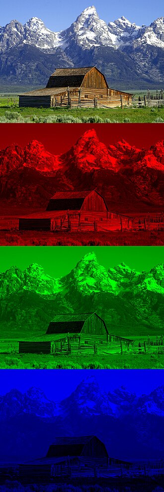
By Mike1024 at English Wikipedia. - Transferred from en.wikipedia to Commons. Transfer was stated to be made by User:nopira., Public Domain, Link

Satellite sensors are not limited to visible light. Sentinel-2 measures reflected radiation at several wavelength ranges, including visible light, near-infrared (NIR), and short-wave infrared (SWIR). Each measured wavelength range is stored as a separate spectral band. Different materials interact with electromagnetic radiation differently. For example, healthy vegetation strongly reflects near-infrared radiation, while water absorbs much of it. Some differences that are difficult to observe in an RGB image therefore become much clearer when additional spectral bands are available. Sentinel-2 contains the following 13 bands:

Band	Region	Approx. central wavelength	Spatial resolution
B1	Coastal aerosol	443 nm	60 m
B2	Blue	490 nm	10 m
B3	Green	560 nm	10 m
B4	Red	665 nm	10 m
B5	Red edge	705 nm	20 m
B6	Red edge	740 nm	20 m
B7	Red edge	783 nm	20 m
B8	Near-infrared	842 nm	10 m
B8A	Narrow near-infrared	865 nm	20 m
B9	Water vapour	945 nm	60 m
B10	Cirrus	1375 nm	60 m
B11	Short-wave infrared	1610 nm	20 m
B12	Short-wave infrared	2190 nm	20 m

Notice that the bands do not all have the same spatial resolution. Sentinel-2 measures some bands at $10$ m, others at $20$ m, and others at $60$ m. We will return to this issue later when discussing spatial resolution and preprocessing. EuroSAT provides all 13 bands as channels of the same sample, allowing us to inspect information that would be completely absent from an ordinary RGB image.

In [6]:

dataset.bands

dataset.bands

Out[6]:

('B01',
 'B02',
 'B03',
 'B04',
 'B05',
 'B06',
 'B07',
 'B08',
 'B09',
 'B10',
 'B11',
 'B12',
 'B8A')

Exercise

Extract the red band (B04) from the current image.

In [ ]:

# 1. Find the index of B04 in dataset.bands.
# 2. Use the index to select B04 from image.

# 1. Find the index of B04 in dataset.bands. # 2. Use the index to select B04 from image.

In [11]:

# @title
red_index = dataset.bands.index("B04")
sample['image'][red_index]

# @title red_index = dataset.bands.index("B04") sample['image'][red_index]

Out[11]:

tensor([[1531., 1531., 1498.,  ..., 1459., 1461., 1481.],
        [1531., 1531., 1498.,  ..., 1459., 1461., 1481.],
        [1526., 1526., 1455.,  ..., 1444., 1470., 1462.],
        ...,
        [1125., 1125., 1174.,  ..., 1184., 1307., 1359.],
        [1149., 1149., 1187.,  ..., 1153., 1365., 1444.],
        [1196., 1196., 1189.,  ..., 1063., 1233., 1291.]])

Hence, dataset[0]["image"][0] corresponds to B01 channel of the first image, dataset[50]["image"][1] to B02 channel of the 51th image, and so on. Lets first inspect several individual bands separately. Since a single spectral band contains one measurement per pixel, it can be visualized as a grayscale image. Brighter pixels indicate larger values in that band, while darker pixels indicate smaller values. We will compare the blue, red, near-infrared, and short-wave infrared bands. The same geographical area can appear quite different in each one because different surface materials reflect different amounts of radiation at different wavelengths.

In [12]:

import matplotlib.pyplot as plt

image = sample["image"]
band_names = ["B02", "B04", "B08", "B11"]

fig, axes = plt.subplots(1, 4, figsize=(14, 4))
for ax, band in zip(axes, band_names):
    index = dataset.bands.index(band)
    ax.imshow(image[index], cmap="gray")
    ax.set_title(band)
    ax.axis("off")
plt.show()

import matplotlib.pyplot as plt image = sample["image"] band_names = ["B02", "B04", "B08", "B11"] fig, axes = plt.subplots(1, 4, figsize=(14, 4)) for ax, band in zip(axes, band_names): index = dataset.bands.index(band) ax.imshow(image[index], cmap="gray") ax.set_title(band) ax.axis("off") plt.show()

A normal RGB image combines three channels corresponding approximately to red, green, and blue light. We can construct a similar true-color composite from Sentinel-2 using red (B04), green (B03), and blue (B02). These three bands are combined into a three-channel image so that the result resembles what we would expect to see with human vision.

However, the raw satellite values are not necessarily suitable for direct display. The reflectance values of different bands can occupy different numerical ranges. We therefore stretch each RGB channel independently using its lower and upper percentiles. This improves contrast and produces a more natural-looking image. This operation is only for visualization and should not be confused with normalization used when training a neural network.

In [13]:

import torch

rgb_indices = [dataset.bands.index(band) for band in ["B04", "B03", "B02"]]
rgb = image[rgb_indices].float()

for c in range(3):
    low = torch.quantile(rgb[c], 0.02)
    high = torch.quantile(rgb[c], 0.98)
    rgb[c] = (rgb[c] - low) / (high - low)

rgb = rgb.clamp(0, 1)

plt.figure(figsize=(5, 5))
plt.imshow(rgb.permute(1, 2, 0))
plt.axis("off")
plt.show()

import torch rgb_indices = [dataset.bands.index(band) for band in ["B04", "B03", "B02"]] rgb = image[rgb_indices].float() for c in range(3): low = torch.quantile(rgb[c], 0.02) high = torch.quantile(rgb[c], 0.98) rgb[c] = (rgb[c] - low) / (high - low) rgb = rgb.clamp(0, 1) plt.figure(figsize=(5, 5)) plt.imshow(rgb.permute(1, 2, 0)) plt.axis("off") plt.show()

The remaining bands contain information outside human vision. Instead of ignoring them, we can deliberately map some of these invisible wavelengths to visible colors. This produces a false-color composite, which can make particular surface properties much easier to distinguish. A common Sentinel-2 false-color combination uses B08, B04, B03. Vegetation reflects strongly in the NIR band B08. Since B08 is displayed as red in this composite, vegetated areas usually appear bright red.

In [14]:

false_indices = [dataset.bands.index(band) for band in ["B08", "B04", "B03"]]
false_color = image[false_indices].float()

for c in range(3):
    low = torch.quantile(false_color[c], 0.02)
    high = torch.quantile(false_color[c], 0.98)
    false_color[c] = (false_color[c] - low) / (high - low)

false_color = false_color.clamp(0, 1)

fig, axes = plt.subplots(1, 2, figsize=(10, 4))

axes[0].imshow(rgb.permute(1, 2, 0))
axes[0].set_title("True Color")
axes[0].axis("off")

axes[1].imshow(false_color.permute(1, 2, 0))
axes[1].set_title("False Color (B08, B04, B03)")
axes[1].axis("off")

plt.show()

false_indices = [dataset.bands.index(band) for band in ["B08", "B04", "B03"]] false_color = image[false_indices].float() for c in range(3): low = torch.quantile(false_color[c], 0.02) high = torch.quantile(false_color[c], 0.98) false_color[c] = (false_color[c] - low) / (high - low) false_color = false_color.clamp(0, 1) fig, axes = plt.subplots(1, 2, figsize=(10, 4)) axes[0].imshow(rgb.permute(1, 2, 0)) axes[0].set_title("True Color") axes[0].axis("off") axes[1].imshow(false_color.permute(1, 2, 0)) axes[1].set_title("False Color (B08, B04, B03)") axes[1].axis("off") plt.show()

Normalized Difference Vegatation Index (NDVI)¶

A common example of how we can use the additional bands further can be demonstrated with the Normalized Difference Vegetation Index (NDVI). Healthy vegetation typically absorbs much of the visible red light for photosynthesis while reflecting strongly in the near-infrared region. We can therefore compare the near-infrared and red bands:

$$ \mathrm{NDVI} = \frac{\mathrm{NIR} - \mathrm{Red}} {\mathrm{NIR} + \mathrm{Red}} $$

NDVI values theoretically range from $-1$ to $1$. Larger positive values generally indicate stronger vegetation response, while values around zero or below are commonly associated with surfaces such as water, bare ground, or built-up areas. NDVI is not a vegetation classifier by itself, but it provides a simple example of how spectral information that is invisible in an RGB image can be converted into useful information.

Exercise

Calculate the NDVI values for the current image.

In [ ]:

# 1. Extract the near-infrared band (B08).
# 2. Extract the red band (B04).
# 3. Calculate NDVI.

# 1. Extract the near-infrared band (B08). # 2. Extract the red band (B04). # 3. Calculate NDVI.

In [15]:

# @title
nir = image[dataset.bands.index("B08")].float()
red = image[dataset.bands.index("B04")].float()
ndvi = (nir - red) / (nir + red + 1e-6)

# @title nir = image[dataset.bands.index("B08")].float() red = image[dataset.bands.index("B04")].float() ndvi = (nir - red) / (nir + red + 1e-6)

In [16]:

fig, axes = plt.subplots(1, 2, figsize=(10, 4))

axes[0].imshow(rgb.permute(1, 2, 0))
axes[0].set_title("True Color")
axes[0].axis("off")

im = axes[1].imshow(ndvi, cmap="RdYlGn", vmin=-1, vmax=1)
axes[1].set_title("NDVI")
axes[1].axis("off")

fig.colorbar(im, ax=axes[1], fraction=0.046, pad=0.04)

plt.show()

fig, axes = plt.subplots(1, 2, figsize=(10, 4)) axes[0].imshow(rgb.permute(1, 2, 0)) axes[0].set_title("True Color") axes[0].axis("off") im = axes[1].imshow(ndvi, cmap="RdYlGn", vmin=-1, vmax=1) axes[1].set_title("NDVI") axes[1].axis("off") fig.colorbar(im, ax=axes[1], fraction=0.046, pad=0.04) plt.show()

The NDVI map assigns a continuous value to each pixel. We can convert it into a simple binary mask by choosing a threshold. For example, we may classify pixels with $\mathrm{NDVI} > 0.3$ as vegetation. A suitable threshold value depends on the location, season, vegetation type, atmospheric conditions, and preprocessing.

Exercise

Create a vegetation mask using NDVI > 0.3.

In [17]:

# Your code here.

# Your code here.

In [18]:

# @title
vegetation = ndvi > 0.3

# @title vegetation = ndvi > 0.3

In [19]:

fig, axes = plt.subplots(1, 3, figsize=(14, 4))

axes[0].imshow(rgb.permute(1, 2, 0))
axes[0].set_title("True Color")
axes[0].axis("off")

im = axes[1].imshow(ndvi, cmap="RdYlGn", vmin=-1, vmax=1)
axes[1].set_title("NDVI")
axes[1].axis("off")

axes[2].imshow(vegetation, cmap="gray")
axes[2].set_title("NDVI > 0.3")
axes[2].axis("off")

plt.show()

fig, axes = plt.subplots(1, 3, figsize=(14, 4)) axes[0].imshow(rgb.permute(1, 2, 0)) axes[0].set_title("True Color") axes[0].axis("off") im = axes[1].imshow(ndvi, cmap="RdYlGn", vmin=-1, vmax=1) axes[1].set_title("NDVI") axes[1].axis("off") axes[2].imshow(vegetation, cmap="gray") axes[2].set_title("NDVI > 0.3") axes[2].axis("off") plt.show()

GeoTIFF and Rasterio¶

Satellite imagery is commonly stored as raster data. A raster represents an area as a regular grid of pixels, where each pixel stores one or more numerical measurements. A familiar image format such as JPEG or PNG also stores pixels on a grid, but satellite imagery usually requires additional information. In addition to the pixel values themselves, we may need to know:

• where the image is located on the Earth,
• the geographic size represented by each pixel,
• the coordinate reference system,
• which spectral band each channel represents,
• whether some pixels contain missing or invalid data.

One of the most common formats for this purpose is GeoTIFF. A GeoTIFF is a TIFF image that also stores geospatial metadata. This allows software to determine where the raster belongs geographically and how image coordinates correspond to locations on the Earth.

A satellite product may be stored in different ways. For example, each spectral band may be stored in a separate GeoTIFF file, or several bands may be combined into a single multiband GeoTIFF. Other formats are also common. Sentinel-2 products, for example, often store individual bands as JPEG 2000 (.jp2) files inside a larger product structure together with metadata. For machine learning datasets, these source products are frequently converted into simpler GeoTIFF-based representations.

In [20]:

from pathlib import Path

tif_files = list(Path("data").rglob("*.tif"))
tif_files[:5]

from pathlib import Path tif_files = list(Path("data").rglob("*.tif")) tif_files[:5]

Out[20]:

[PosixPath('data/ds/images/remote_sensing/otherDatasets/sentinel_2/tif/Highway/Highway_284.tif'),
 PosixPath('data/ds/images/remote_sensing/otherDatasets/sentinel_2/tif/Highway/Highway_139.tif'),
 PosixPath('data/ds/images/remote_sensing/otherDatasets/sentinel_2/tif/Highway/Highway_2329.tif'),
 PosixPath('data/ds/images/remote_sensing/otherDatasets/sentinel_2/tif/Highway/Highway_2093.tif'),
 PosixPath('data/ds/images/remote_sensing/otherDatasets/sentinel_2/tif/Highway/Highway_280.tif')]

In [21]:

len(tif_files)

len(tif_files)

Out[21]:

27000

TorchGeo loads the EuroSAT samples for us, but it is useful to inspect the underlying raster file directly. A common Python library for working with geospatial rasters is Rasterio. It can read the pixel values together with metadata such as the number of bands, image dimensions, coordinate reference system, geographic bounds, and the transformation between pixel coordinates and geographic coordinates. Lets open one of the EuroSAT GeoTIFF files and inspect this information. Note that unlike geotiff, rasterio is shipped with Google Colab.

In [22]:

import rasterio

tif_path = tif_files[0]

with rasterio.open(tif_path) as src:
    print("File:", tif_path)
    print("Bands:", src.count)
    print("Width:", src.width)
    print("Height:", src.height)
    print("Data type:", src.dtypes)
    print("CRS:", src.crs)
    print("Bounds:", src.bounds)
    print("Transform:", src.transform)

import rasterio tif_path = tif_files[0] with rasterio.open(tif_path) as src: print("File:", tif_path) print("Bands:", src.count) print("Width:", src.width) print("Height:", src.height) print("Data type:", src.dtypes) print("CRS:", src.crs) print("Bounds:", src.bounds) print("Transform:", src.transform)

File: data/ds/images/remote_sensing/otherDatasets/sentinel_2/tif/Highway/Highway_284.tif
Bands: 13
Width: 64
Height: 64
Data type: ('uint16', 'uint16', 'uint16', 'uint16', 'uint16', 'uint16', 'uint16', 'uint16', 'uint16', 'uint16', 'uint16', 'uint16', 'uint16')
CRS: EPSG:32630
Bounds: BoundingBox(left=474297.249073, bottom=4488889.324762307, right=474941.73523736367, top=4489530.63939)
Transform: | 10.07, 0.00, 474297.25|
| 0.00,-10.02, 4489530.64|
| 0.00, 0.00, 1.00|

This raster contains 13 bands and has spatial dimensions of $64 \times 64$ pixels. All bands are stored as uint16, which means that the pixel values are stored as 16-bit unsigned integers. The CRS value printed above identifies the raster's coordinate reference system. For a projected CRS such as UTM, coordinates and pixel sizes are typically expressed in metres. The Transform matrix tells us how to convert between pixel positions and coordinates in that CRS. The Bounds field describes the raster's geographic extent with left, right, bottom, and top values. Because tif_files[0] may select a tile from a different location, the exact CRS, bounds, and pixel size should be read from the Rasterio output rather than assumed in advance.

In [23]:

with rasterio.open(tif_path) as src:
    row, col = 32, 32
    x, y = src.xy(row, col)

print("Pixel:", (row, col))
print("Coordinate:", (x, y))

with rasterio.open(tif_path) as src: row, col = 32, 32 x, y = src.xy(row, col) print("Pixel:", (row, col)) print("Coordinate:", (x, y))

Pixel: (32, 32)
Coordinate: (np.float64(474624.5272033409), np.float64(4489204.971805625))

Rasterio can use the stored geospatial transform to convert any pixel location into coordinates in the raster's CRS. The reverse operation is also possible: given a geographic coordinate, we can determine which raster pixel contains that location.

In [24]:

with rasterio.open(tif_path) as src:
    row, col = src.index(x, y)

print("Recovered pixel:", (row, col))

with rasterio.open(tif_path) as src: row, col = src.index(x, y) print("Recovered pixel:", (row, col))

Recovered pixel: (32, 32)

Coordinate Reference Systems (CRS)¶

The Earth is three-dimensional, while satellite images are stored on a two-dimensional grid. A coordinate reference system (CRS), or spatial reference system, defines how locations on the Earth are represented using numerical coordinates.

A common geographic coordinate system is latitude and longitude, where positions are expressed in degrees. However, distances measured directly in degrees are inconvenient for many image-processing tasks. Projected coordinate systems instead represent the Earth's surface on a two-dimensional plane. The Universal Transverse Mercator (UTM) system is a common example. It divides the Earth into zones and represents locations within each zone using coordinates measured approximately in metres.

By Krishnavedala, CC BY-SA 3.0, Wikimedia Commons.

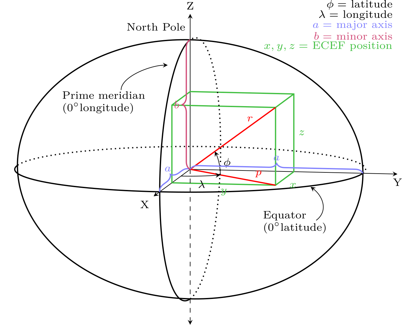
By Krishnavedala, CC BY-SA 3.0, Link

The EuroSAT files may use different projected CRS values depending on where each tile is located. The code below prints the CRS for the selected raster, while src.res reports its pixel size in the units of that CRS. Different satellite images may use different CRS. Before combining images from different sources, we therefore need to ensure that their coordinate systems and spatial grids are compatible.

In [25]:

with rasterio.open(tif_path) as src:
    print(src.crs)
    print(src.res)

with rasterio.open(tif_path) as src: print(src.crs) print(src.res)

EPSG:32630
(10.070096318182275, 10.02054105769807)

Exercise

Calculate the raster width and height in CRS units.

In [26]:

# Use src.width, src.height, and src.res.

# Use src.width, src.height, and src.res.

In [27]:

# @title
with rasterio.open(tif_path) as src:
    raster_width = src.width * src.res[0]
    raster_height = src.height * src.res[1]

print("Raster width:", raster_width)
print("Raster height:", raster_height)

# @title with rasterio.open(tif_path) as src: raster_width = src.width * src.res[0] raster_height = src.height * src.res[1] print("Raster width:", raster_width) print("Raster height:", raster_height)

Raster width: 644.4861643636656
Raster height: 641.3146276926765

Large Satellite Images¶

EuroSAT is convenient for learning how multispectral data are represented, but its images are already small $64 \times 64$ patches. Real satellite products are usually much larger and may cover thousands of pixels in each spatial dimension. Deep learning models usually do not process such large rasters directly. Instead, the image is divided into smaller patches, for example $128 \times 128$, $256 \times 256$, or $512 \times 512$ pixels. Patches may be non-overlapping, or they may overlap. Overlapping patches can reduce boundary artifacts during reconstruction or segmentation, but they also increase the amount of computation. Patching is useful for several reasons:

• large rasters may not fit into GPU memory,
• neural networks usually expect fixed-size inputs,
• one large scene can be converted into many training samples,
• patches can be processed independently during training or inference,
• only selected parts of a large raster need to be loaded when using window-based reading.

EuroSAT is a curated classification dataset in which the original satellite imagery has already been divided into small $64 \times 64$ samples. To see how patch extraction works on a more realistic raster, we will temporarily use a larger Landsat dataset provided by TorchGeo called IOBench, which contains a Landsat 9 scene together with land-cover information. The dataset is relatively large to download.

In [28]:

from torchgeo.datasets import IOBench

large_dataset = IOBench(root="data/iobench", split="preprocessed", download=True)

from torchgeo.datasets import IOBench large_dataset = IOBench(root="data/iobench", split="preprocessed", download=True)

preprocessed.tar.gz: 100%|██████████| 694M/694M [00:08<00:00, 83.5MB/s]

Random and Grid Sampling¶

There are two common ways to extract patches from a large satellite scene. During training, we often want many different samples from different parts of the image. In this case, random sampling is useful. TorchGeo's RandomPatchSampler randomly selects geographic regions from the dataset.

In [39]:

from torchgeo.samplers import RandomPatchSampler

sampler = RandomPatchSampler(large_dataset, size=256, length=10)

bbox = next(iter(sampler))
bbox

from torchgeo.samplers import RandomPatchSampler sampler = RandomPatchSampler(large_dataset, size=256, length=10) bbox = next(iter(sampler)) bbox

Out[39]:

(slice(350340.0, 358020.0, None), slice(4390680.0, 4398360.0, None))

In [30]:

patch = large_dataset[bbox]
patch.keys()

patch = large_dataset[bbox] patch.keys()

Out[30]:

dict_keys(['bounds', 'transform', 'image', 'mask'])

In [31]:

patch['image'].shape

patch['image'].shape

Out[31]:

torch.Size([8, 256, 256])

For evaluation or full-scene prediction, however, we usually want to cover the entire raster systematically. In this case, we can use a grid sampler, which moves across the scene using a fixed patch size and stride. If the stride is equal to the patch size, the patches do not overlap. If the stride is smaller than the patch size, neighbouring patches overlap.

Exercise

Apply grid sampling.

In [32]:

# 1. Import GriddedPatchSampler and sample the dataset with a fixed size of 256.
# 2. Use overlapping and non-overlapping striding and inspect patches.

# 1. Import GriddedPatchSampler and sample the dataset with a fixed size of 256. # 2. Use overlapping and non-overlapping striding and inspect patches.

In [38]:

# @title
from torchgeo.samplers import GriddedPatchSampler

non_overlapping_sampler = GriddedPatchSampler(large_dataset, size=256, stride=256)
overlapping_sampler = GriddedPatchSampler(large_dataset, size=256, stride=128)

non_overlapping_bbox = next(iter(non_overlapping_sampler))
overlapping_bbox = next(iter(overlapping_sampler))

non_overlapping_patch = large_dataset[non_overlapping_bbox]
overlapping_patch = large_dataset[overlapping_bbox]

print("Non-overlapping patch shape:", non_overlapping_patch["image"].shape)
print("Overlapping patch shape:", overlapping_patch["image"].shape)
print("Number of non-overlapping patches:", len(non_overlapping_sampler))
print("Number of overlapping patches:", len(overlapping_sampler))

# @title from torchgeo.samplers import GriddedPatchSampler non_overlapping_sampler = GriddedPatchSampler(large_dataset, size=256, stride=256) overlapping_sampler = GriddedPatchSampler(large_dataset, size=256, stride=128) non_overlapping_bbox = next(iter(non_overlapping_sampler)) overlapping_bbox = next(iter(overlapping_sampler)) non_overlapping_patch = large_dataset[non_overlapping_bbox] overlapping_patch = large_dataset[overlapping_bbox] print("Non-overlapping patch shape:", non_overlapping_patch["image"].shape) print("Overlapping patch shape:", overlapping_patch["image"].shape) print("Number of non-overlapping patches:", len(non_overlapping_sampler)) print("Number of overlapping patches:", len(overlapping_sampler))

Non-overlapping patch shape: torch.Size([8, 256, 256])
Overlapping patch shape: torch.Size([8, 256, 256])
Number of non-overlapping patches: 992
Number of overlapping patches: 3782

Preprocessing Satellite Images¶

Before satellite imagery is passed to a neural network, the raw pixel values usually need to be transformed into a more suitable numerical representation. The exact preprocessing depends on the sensor and dataset, but several operations are common:

• selecting the spectral bands required by the task,
• converting integer pixel values to floating-point values,
• scaling or normalizing the bands,
• handling missing or invalid pixels,
• resampling bands when their spatial resolutions differ,
• extracting fixed-size patches,
• applying data augmentation during training.

One important point is that visualization scaling and model normalization are not the same operation. Earlier, we used percentile stretching to make RGB and false-color images easier to display. That transformation changes the image for human viewing. For neural networks, normalization should instead be defined consistently across the training dataset.

Band-wise Normalization¶

Different spectral bands can have different numerical distributions. Treating all channels identically may therefore be inappropriate. A common approach is to calculate a mean and standard deviation for each band across the training dataset and normalize each channel separately:

$$ x^{\prime}_c = \frac{x_c - \mu_c}{\sigma_c} $$

where $\mu_c$ and $\sigma_c$ are the mean and standard deviation of band $c$. This is analogous to channel-wise normalization for RGB images, but a multispectral image may require statistics for many more channels.

In [33]:

image = sample["image"].float()

for band_name in ["B02", "B03", "B04", "B08"]:
    idx = dataset.bands.index(band_name)
    band = image[idx]

    print(
        band_name,
        "min =", band.min().item(),
        "max =", band.max().item(),
        "mean =", band.mean().item()
    )

image = sample["image"].float() for band_name in ["B02", "B03", "B04", "B08"]: idx = dataset.bands.index(band_name) band = image[idx] print( band_name, "min =", band.min().item(), "max =", band.max().item(), "mean =", band.mean().item() )

B02 min = 1045.0 max = 1894.0 mean = 1287.623779296875
B03 min = 979.0 max = 2144.0 mean = 1379.360595703125
B04 min = 845.0 max = 2935.0 mean = 1498.05419921875
B08 min = 1649.0 max = 4840.0 mean = 3358.2861328125

Exercise

Normalize each band of the current image independently.

In [34]:

# Your code here.

# Your code here.

In [35]:

# @title
normalized = image.clone()

for c in range(image.shape[0]):
    mean = image[c].mean()
    std = image[c].std()
    normalized[c] = (image[c] - mean) / (std + 1e-6)

# @title normalized = image.clone() for c in range(image.shape[0]): mean = image[c].mean() std = image[c].std() normalized[c] = (image[c] - mean) / (std + 1e-6)

In [36]:

for c in range(4):
    print(
        dataset.bands[c],
        "mean =", normalized[c].mean().item(),
        "std =", normalized[c].std().item()
    )

for c in range(4): print( dataset.bands[c], "mean =", normalized[c].mean().item(), "std =", normalized[c].std().item() )

B01 mean = -4.190951585769653e-09 std = 1.0
B02 mean = 3.026798367500305e-09 std = 1.0
B03 mean = -1.6298145055770874e-09 std = 1.0
B04 mean = -9.313225746154785e-10 std = 1.0

The previous example calculates the statistics from a single image only to demonstrate the operation. For an actual deep learning pipeline, the mean and standard deviation should normally be estimated from the training dataset and then reused for the test set. Computing separate statistics from the test data would allow information from the evaluation set to influence preprocessing.

Resampling Bands with Different Spatial Resolutions¶

Sentinel-2 bands are not all acquired at the same spatial resolution. Some bands are provided at $10$ m, others at $20$ m, and others at $60$ m. This creates a practical problem, as a neural network usually expects the channels of one input tensor to have the same spatial dimensions. Suppose one band has shape $H \times W$ while another band covering the same geographic area has shape $\frac{H}{2} \times \frac{W}{2}.$ Before stacking them into a single tensor, the bands need to be placed on a common spatial grid. This is usually done through resampling. Common resampling methods include:

• nearest-neighbour interpolation,
• bilinear interpolation,
• cubic interpolation.

Nearest-neighbour interpolation is often used for categorical data such as masks or land-cover labels, because it does not create intermediate class values. Bilinear or cubic interpolation is more suitable for continuous-valued imagery. Upsampling a $20$ m band to a $10$ m grid only changes the sampling grid -- it does not make the original measurement equivalent to a true $10$ m observation.

In [40]:

import torch.nn.functional as F

band = image[dataset.bands.index("B05")].float()

small = F.interpolate(
    band.unsqueeze(0).unsqueeze(0),
    size=(32, 32),
    mode="bilinear",
    align_corners=False
).squeeze()

upsampled = F.interpolate(
    small.unsqueeze(0).unsqueeze(0),
    size=(64, 64),
    mode="bilinear",
    align_corners=False
).squeeze()

fig, axes = plt.subplots(1, 2, figsize=(9, 4))

axes[0].imshow(small, cmap="gray")
axes[0].set_title("32 × 32")
axes[0].axis("off")

axes[1].imshow(upsampled, cmap="gray")
axes[1].set_title("Upsampled to 64 × 64")
axes[1].axis("off")

plt.show()

import torch.nn.functional as F band = image[dataset.bands.index("B05")].float() small = F.interpolate( band.unsqueeze(0).unsqueeze(0), size=(32, 32), mode="bilinear", align_corners=False ).squeeze() upsampled = F.interpolate( small.unsqueeze(0).unsqueeze(0), size=(64, 64), mode="bilinear", align_corners=False ).squeeze() fig, axes = plt.subplots(1, 2, figsize=(9, 4)) axes[0].imshow(small, cmap="gray") axes[0].set_title("32 × 32") axes[0].axis("off") axes[1].imshow(upsampled, cmap="gray") axes[1].set_title("Upsampled to 64 × 64") axes[1].axis("off") plt.show()

The second image contains four times as many pixels, but it does not contain four times as much information. The additional pixel values have been estimated from neighbouring measurements through interpolation. Resampling a $20$ m band to a $10$ m grid allows it to be stacked with the $10$ m bands, but it does not turn the original $20$ m observation into a true $10$ m measurement. In practice, multispectral datasets such as EuroSAT may already provide bands resampled to a common grid. When working with original satellite products, however, resolution alignment is often part of the preprocessing pipeline.

Multimodal and Multitemporal Satellite Data¶

In many remote sensing problems, a single satellite image does not contain all the information needed for a task. Instead, we may combine several sources of information about the same geographic region.

When data from different sensors or sensing systems are combined, we refer to this as multimodal data. For example, optical imagery can be combined with radar imagery. Each modality provides different information, so using them together can give a model a more complete description of the observed area. For multimodal processing, the observations should usually correspond to approximately the same geographic region. They may also need to be resampled or aligned to the same spatial resolution and image grid before they can be processed together.

Another common setting is multitemporal data, where the same region is observed at different times. Instead of having only one image of a location, we may have a sequence of images acquired over several days, months, or years. Multitemporal data allows us to observe how the Earth's surface changes over time. It is useful for tasks such as crop monitoring, deforestation detection, flood analysis, urban development, and land-cover change detection.

Multimodal and multitemporal information can also be used together. For example, a model may receive several optical observations from different dates together with radar observations of the same region to remove clouds.

A single multispectral image is usually represented as a tensor with shape $C \times H \times W$, where $C$ is the number of spectral bands and $H$ and $W$ are the spatial dimensions. For multitemporal data, we need an additional dimension representing time. If the same location is observed at three different times, the observations can be stacked into a tensor with shape $T \times C \times H \times W$, where $T=3$ is the number of observations.

For multimodal data, different modalities may contain different numbers of channels. One simple approach is to concatenate them along the channel dimension. For example, four optical bands and two radar channels can be represented together as six channels. This requires the observations to be spatially aligned and to have the same height and width.

To see how multitemporal data is represented in practice, we will use PASTIS100, a subset of the PASTIS dataset where each geographic region contains multiple satellite observations acquired at different times.

In [41]:

from torchgeo.datasets import PASTIS100

pastis_s2 = PASTIS100(root="data/pastis100", bands=PASTIS100.s2_bands, download=True)

from torchgeo.datasets import PASTIS100 pastis_s2 = PASTIS100(root="data/pastis100", bands=PASTIS100.s2_bands, download=True)

PASTIS-R.zip: 100%|██████████| 1.90G/1.90G [01:23<00:00, 24.3MB/s]

In [42]:

sample = pastis_s2[0]
s2 = sample["image"]

print("Time series shape:", s2.shape)
print("Number of observations:", s2.shape[0])
print("Number of bands:", s2.shape[1])
print("Height and width:", s2.shape[2:])

sample = pastis_s2[0] s2 = sample["image"] print("Time series shape:", s2.shape) print("Number of observations:", s2.shape[0]) print("Number of bands:", s2.shape[1]) print("Height and width:", s2.shape[2:])

Time series shape: torch.Size([43, 10, 128, 128])
Number of observations: 43
Number of bands: 10
Height and width: torch.Size([128, 128])

The first dimension now represents different observations through time. The exact number of observations may vary between samples because the satellite does not necessarily provide a usable image of every location on exactly the same dates.

We can visualize a few observations from the sequence. Sentinel-2 contains multiple spectral bands, but for visualization we select the red, green, and blue bands and construct an RGB image in the same way as before. The important point here is that all of the images below correspond to the same geographic region, but were acquired at different times. Differences between them may therefore represent seasonal changes, changes in vegetation, atmospheric conditions, or actual changes on the ground.

In [43]:

fig, axes = plt.subplots(3, 3, figsize=(10, 10))

indices = range(1, 10)

for ax, t in zip(axes.flat, indices):
    rgb = s2[t, [2, 1, 0]].permute(1, 2, 0)

    rgb = rgb / 5000
    rgb = rgb.clamp(0, 1)

    ax.imshow(rgb)
    ax.set_title(f"Observation {t}")
    ax.axis("off")

plt.tight_layout()
plt.show()

fig, axes = plt.subplots(3, 3, figsize=(10, 10)) indices = range(1, 10) for ax, t in zip(axes.flat, indices): rgb = s2[t, [2, 1, 0]].permute(1, 2, 0) rgb = rgb / 5000 rgb = rgb.clamp(0, 1) ax.imshow(rgb) ax.set_title(f"Observation {t}") ax.axis("off") plt.tight_layout() plt.show()

The same PASTIS data also contains Sentinel-1 radar observations. We saw that Sentinel-2 provides multispectral optical observations, while Sentinel-1 provides radar observations. The two modalities therefore have different numbers of channels and measure different properties of the surface.

We should also not assume that the Sentinel-1 and Sentinel-2 observations were acquired at exactly the same times. In real multimodal satellite datasets, different sensors often have different acquisition schedules. As a result, the number of observations in the two time series may also be different.

Exercise

Load Pastis100 S1 data and print a sample shape

In [ ]:

# Your code here.

# Your code here.

In [44]:

# @title
pastis_s1 = PASTIS100(root="data/pastis100", bands=PASTIS100.s1a_bands, download=False)

s1 = pastis_s1[0]["image"]
s2 = pastis_s2[0]["image"]

print("Sentinel-2 time series:", s2.shape)
print("Sentinel-1 time series:", s1.shape)

# @title pastis_s1 = PASTIS100(root="data/pastis100", bands=PASTIS100.s1a_bands, download=False) s1 = pastis_s1[0]["image"] s2 = pastis_s2[0]["image"] print("Sentinel-2 time series:", s2.shape) print("Sentinel-1 time series:", s1.shape)

Sentinel-2 time series: torch.Size([43, 10, 128, 128])
Sentinel-1 time series: torch.Size([65, 3, 128, 128])

Before combining the modalities observation-by-observation, we would need to consider their acquisition dates and determine which observations should be matched. For now, we can inspect several Sentinel-1 observations from the same sample. Unlike an RGB image, radar data cannot be displayed directly as natural colors. We will visualize one radar channel as a grayscale image.

In [45]:

fig, axes = plt.subplots(1, 3, figsize=(12, 4))

indices = [0, 1, 2]

for ax, t in zip(axes, indices):
    radar = s1[t, 0]

    ax.imshow(radar, cmap="gray")
    ax.set_title(f"Observation {t + 1}")
    ax.axis("off")

plt.tight_layout()
plt.show()

fig, axes = plt.subplots(1, 3, figsize=(12, 4)) indices = [0, 1, 2] for ax, t in zip(axes, indices): radar = s1[t, 0] ax.imshow(radar, cmap="gray") ax.set_title(f"Observation {t + 1}") ax.axis("off") plt.tight_layout() plt.show()

There are several ways to provide such information to a neural network. If observations are spatially and temporally aligned, a simple approach is to concatenate their channels. More complex models may instead process each modality or each timestep separately and combine the resulting features later. The exact fusion strategy depends on the task and the structure of the available data. In the remainder of this notebook, we will return to a simpler single-image setting and use satellite imagery to train a neural network for a LULC classification task.

Land-use Land-cover Classification with ConvNet¶

One common application of satellite imagery is land-use and land-cover (LULC) classification. The goal is to assign an image, or sometimes each individual pixel, to a class describing the type or use of the observed area. Examples of classes include forests, agricultural land, residential areas, industrial areas, rivers, and highways. In this notebook, we will consider image-level classification, where each satellite image receives one class label.

Loading Satellite Data¶

We will reuse the EuroSAT dataset introduced earlier. We will prepare the images, use the predefined training and test splits, and train a small convolutional neural network to predict the land-cover class. EuroSAT provides predefined splits in TorchGeo. We will use the training and test splits for simplicity. For the first classification experiment, we will use all 13 Sentinel-2 bands which means that the input to our neural network will have shape $13 \times 64 \times 64$.

In [46]:

train_dataset = EuroSAT(root="data", split="train", download=False)
test_dataset = EuroSAT(root="data", split="test", download=True)

print("Training samples:", len(train_dataset))
print("Test samples:", len(test_dataset))

print("Image shape:", train_dataset[0]["image"].shape)
print("Number of classes:", len(train_dataset.classes))
print("Classes:", train_dataset.classes)

train_dataset = EuroSAT(root="data", split="train", download=False) test_dataset = EuroSAT(root="data", split="test", download=True) print("Training samples:", len(train_dataset)) print("Test samples:", len(test_dataset)) print("Image shape:", train_dataset[0]["image"].shape) print("Number of classes:", len(train_dataset.classes)) print("Classes:", train_dataset.classes)

eurosat-test.txt: 100%|██████████| 102k/102k [00:00<00:00, 9.79MB/s]

Training samples: 16200
Test samples: 5400
Image shape: torch.Size([13, 64, 64])
Number of classes: 10
Classes: ['AnnualCrop', 'Forest', 'HerbaceousVegetation', 'Highway', 'Industrial', 'Pasture', 'PermanentCrop', 'Residential', 'River', 'SeaLake']

PyTorch provides the DataLoader class which groups samples into batches and can also shuffle the training data between epochs. We will use a moderate batch size and create separate data loaders for the training and test splits.

In [47]:

from torch.utils.data import DataLoader

batch_size = 64

train_loader = DataLoader(train_dataset, batch_size=batch_size, shuffle=True)
test_loader = DataLoader(test_dataset, batch_size=batch_size, shuffle=False)

batch = next(iter(train_loader))

print("Image batch shape:", batch["image"].shape)
print("Label batch shape:", batch["label"].shape)

from torch.utils.data import DataLoader batch_size = 64 train_loader = DataLoader(train_dataset, batch_size=batch_size, shuffle=True) test_loader = DataLoader(test_dataset, batch_size=batch_size, shuffle=False) batch = next(iter(train_loader)) print("Image batch shape:", batch["image"].shape) print("Label batch shape:", batch["label"].shape)

Image batch shape: torch.Size([64, 13, 64, 64])
Label batch shape: torch.Size([64])

Exercise

Store the batch size, number of bands, height, and width in separate variables.

In [ ]:

# Read the four dimensions from batch["image"].shape.

# Read the four dimensions from batch["image"].shape.

In [48]:

# @title
batch_size, num_bands, height, width = batch["image"].shape

print("Batch size:", batch_size)
print("Number of bands:", num_bands)
print("Height:", height)
print("Width:", width)

# @title batch_size, num_bands, height, width = batch["image"].shape print("Batch size:", batch_size) print("Number of bands:", num_bands) print("Height:", height) print("Width:", width)

Batch size: 64
Number of bands: 13
Height: 64
Width: 64

The image batch now has shape $B \times C \times H \times W$. Here, $B$ is the batch size, while the remaining dimensions correspond to the 13 spectral bands and the spatial dimensions of each EuroSAT image. The labels form a one-dimensional tensor containing one class index for each image in the batch. These image-label pairs are what we will provide to the neural network during training.

Preprocessing Satellite Data¶

Before defining the model, we still need one important preprocessing step. Instead of normalizing every image independently, we should estimate one mean and standard deviation for each spectral band from the training set and reuse these statistics for both dataset splits. As discussed earlier, the spectral bands have different numerical ranges and distributions. Before training the CNN, we will normalize each band using statistics calculated from the training data.

It is important that these statistics are calculated only from the training set. The same mean and standard deviation will then be applied to the test set. This avoids using information from the test data during training.

In [49]:

num_bands = 13

band_sum = torch.zeros(num_bands)
band_squared_sum = torch.zeros(num_bands)
num_pixels = 0

for batch in train_loader:
    images = batch["image"].float()

    band_sum += images.sum(dim=(0, 2, 3))
    band_squared_sum += (images ** 2).sum(dim=(0, 2, 3))

    num_pixels += images.shape[0] * images.shape[2] * images.shape[3]

band_mean = band_sum / num_pixels
band_std = torch.sqrt(
    band_squared_sum / num_pixels - band_mean ** 2
)

print("Band means:")
print(band_mean)

print("\nBand standard deviations:")
print(band_std)

num_bands = 13 band_sum = torch.zeros(num_bands) band_squared_sum = torch.zeros(num_bands) num_pixels = 0 for batch in train_loader: images = batch["image"].float() band_sum += images.sum(dim=(0, 2, 3)) band_squared_sum += (images ** 2).sum(dim=(0, 2, 3)) num_pixels += images.shape[0] * images.shape[2] * images.shape[3] band_mean = band_sum / num_pixels band_std = torch.sqrt( band_squared_sum / num_pixels - band_mean ** 2 ) print("Band means:") print(band_mean) print("\nBand standard deviations:") print(band_std)

Band means:
tensor([1354.4055, 1118.2443, 1042.9299,  947.6262, 1199.4730, 1999.7909,
        2369.2236, 2296.8259,  732.0833,   12.1133, 1819.0104, 1118.9241,
        2594.1404])

Band standard deviations:
tensor([ 245.7173,  333.0071,  395.0921,  593.7506,  566.4172,  861.1838,
        1086.6288, 1117.9821,  404.9200,    4.7759, 1002.5868,  761.3033,
        1231.5878])

We can now use the calculated statistics to normalize every EuroSAT image before it is passed to the neural network. For each spectral band, we subtract its training-set mean and divide by its training-set standard deviation.

The same normalization must be applied to the training and test sets. Only the statistics come from the training set. PyTorch / TorchGeo datasets accept a transform that is applied whenever a sample is loaded. We will define a small transform that converts the image to floating point values and performs band-wise normalization.

In [50]:

def normalize_sample(sample):
    image = sample["image"].float()
    image = (image - band_mean[:, None, None]) / band_std[:, None, None]
    sample["image"] = image
    return sample

def normalize_sample(sample): image = sample["image"].float() image = (image - band_mean[:, None, None]) / band_std[:, None, None] sample["image"] = image return sample

In [51]:

train_dataset = EuroSAT(root="data", split="train", transforms=normalize_sample, download=False)
test_dataset = EuroSAT(root="data", split="test", transforms=normalize_sample, download=False)

train_loader = DataLoader(train_dataset, batch_size=batch_size, shuffle=True)
test_loader = DataLoader(test_dataset, batch_size=batch_size, shuffle=False)

train_dataset = EuroSAT(root="data", split="train", transforms=normalize_sample, download=False) test_dataset = EuroSAT(root="data", split="test", transforms=normalize_sample, download=False) train_loader = DataLoader(train_dataset, batch_size=batch_size, shuffle=True) test_loader = DataLoader(test_dataset, batch_size=batch_size, shuffle=False)

CNN Architecture¶

We will now define a small Convolutional Neural Network (CNN) for LULC classification. The purpose here is to create a simple architecture that allows us to follow the complete training and evaluation pipeline.

The network receives a $13 \times 64 \times 64$ multispectral image. Convolutional layers extract local spatial patterns from the image, while pooling layers gradually reduce the spatial dimensions. As the image passes through deeper layers, the network learns increasingly abstract features that can help distinguish between different land-cover classes.

After the convolutional part of the network, we reduce the remaining spatial dimensions to a single feature vector. A final fully connected layer then produces one output value for each EuroSAT class. These outputs will later be converted into class predictions during training and evaluation.

In [52]:

import torch.nn as nn

class SatCNN(nn.Module):
    def __init__(self, num_classes):
        super().__init__()

        self.features = nn.Sequential(
            nn.Conv2d(13, 32, kernel_size=3, padding=1),
            nn.ReLU(),
            nn.MaxPool2d(2),

            nn.Conv2d(32, 64, kernel_size=3, padding=1),
            nn.ReLU(),
            nn.MaxPool2d(2),

            nn.Conv2d(64, 128, kernel_size=3, padding=1),
            nn.ReLU(),
            nn.AdaptiveAvgPool2d(1)
        )

        self.classifier = nn.Linear(128, num_classes)

    def forward(self, x):
        x = self.features(x)
        x = x.flatten(1)
        x = self.classifier(x)
        return x


model = SatCNN(num_classes=len(train_dataset.classes))
print(model)

import torch.nn as nn class SatCNN(nn.Module): def __init__(self, num_classes): super().__init__() self.features = nn.Sequential( nn.Conv2d(13, 32, kernel_size=3, padding=1), nn.ReLU(), nn.MaxPool2d(2), nn.Conv2d(32, 64, kernel_size=3, padding=1), nn.ReLU(), nn.MaxPool2d(2), nn.Conv2d(64, 128, kernel_size=3, padding=1), nn.ReLU(), nn.AdaptiveAvgPool2d(1) ) self.classifier = nn.Linear(128, num_classes) def forward(self, x): x = self.features(x) x = x.flatten(1) x = self.classifier(x) return x model = SatCNN(num_classes=len(train_dataset.classes)) print(model)

SatCNN(
  (features): Sequential(
    (0): Conv2d(13, 32, kernel_size=(3, 3), stride=(1, 1), padding=(1, 1))
    (1): ReLU()
    (2): MaxPool2d(kernel_size=2, stride=2, padding=0, dilation=1, ceil_mode=False)
    (3): Conv2d(32, 64, kernel_size=(3, 3), stride=(1, 1), padding=(1, 1))
    (4): ReLU()
    (5): MaxPool2d(kernel_size=2, stride=2, padding=0, dilation=1, ceil_mode=False)
    (6): Conv2d(64, 128, kernel_size=(3, 3), stride=(1, 1), padding=(1, 1))
    (7): ReLU()
    (8): AdaptiveAvgPool2d(output_size=1)
  )
  (classifier): Linear(in_features=128, out_features=10, bias=True)
)

Before training, it is useful to verify that the model accepts a batch from our data loader and produces an output with the expected dimensions. If the input batch contains $B$ images and EuroSAT contains 10 classes, the output should have shape $B \times 10$. Each row contains the model's scores for the 10 possible classes for one image.

In [53]:

batch = next(iter(train_loader))
images = batch["image"]

outputs = model(images)

print("Input shape:", images.shape)
print("Output shape:", outputs.shape)

batch = next(iter(train_loader)) images = batch["image"] outputs = model(images) print("Input shape:", images.shape) print("Output shape:", outputs.shape)

Input shape: torch.Size([64, 13, 64, 64])
Output shape: torch.Size([64, 10])

Loss Function, Optimizer, and Device¶

To train the network, we need a way to measure how different the model's predictions are from the correct class labels. For a multi-class classification problem such as EuroSAT, we can use cross-entropy loss.

We also need an optimizer to update the model parameters after the loss has been calculated. We will use the AdamW optimizer, which is a common default choice for training neural networks. Finally, we move the model to a GPU if one is available (otherwise training will take quite a time).

In [54]:

import torch.optim as optim

device = torch.device("cuda" if torch.cuda.is_available() else "cpu")

model = model.to(device)
criterion = nn.CrossEntropyLoss()
optimizer = optim.AdamW(model.parameters(),lr=0.001)

print("Device:", device)

import torch.optim as optim device = torch.device("cuda" if torch.cuda.is_available() else "cpu") model = model.to(device) criterion = nn.CrossEntropyLoss() optimizer = optim.AdamW(model.parameters(),lr=0.001) print("Device:", device)

Device: cuda

During training, each batch will pass through the same sequence of steps. First, the images are passed through the CNN to obtain class scores. The loss is then calculated by comparing these scores with the correct labels. Next, PyTorch calculates the gradients of the loss with respect to the model parameters using backpropagation. The optimizer uses these gradients to update the parameters.

Training accuracy tells us how well the network fits the images that were used to update its parameters. After training, we evaluate the model on the separate test set to estimate how well it generalizes to unseen images.

In [55]:

num_epochs = 5

for epoch in range(num_epochs):
    model.train()

    correct = 0
    total = 0
    running_loss = 0.0

    for batch in train_loader:
        images = batch["image"].to(device)
        labels = batch["label"].to(device)

        optimizer.zero_grad()

        outputs = model(images)
        loss = criterion(outputs, labels)

        loss.backward()
        optimizer.step()

        running_loss += loss.item() * images.size(0)

        predictions = outputs.argmax(dim=1)
        correct += (predictions == labels).sum().item()
        total += labels.size(0)

    print(
        f"Epoch {epoch + 1}/{num_epochs} | "
        f"Loss: {running_loss / total:.4f} | "
        f"Accuracy: {correct / total:.4f}"
    )

num_epochs = 5 for epoch in range(num_epochs): model.train() correct = 0 total = 0 running_loss = 0.0 for batch in train_loader: images = batch["image"].to(device) labels = batch["label"].to(device) optimizer.zero_grad() outputs = model(images) loss = criterion(outputs, labels) loss.backward() optimizer.step() running_loss += loss.item() * images.size(0) predictions = outputs.argmax(dim=1) correct += (predictions == labels).sum().item() total += labels.size(0) print( f"Epoch {epoch + 1}/{num_epochs} | " f"Loss: {running_loss / total:.4f} | " f"Accuracy: {correct / total:.4f}" )

Epoch 1/5 | Loss: 0.8808 | Accuracy: 0.6934
Epoch 2/5 | Loss: 0.4835 | Accuracy: 0.8391
Epoch 3/5 | Loss: 0.3894 | Accuracy: 0.8721
Epoch 4/5 | Loss: 0.3353 | Accuracy: 0.8900
Epoch 5/5 | Loss: 0.2868 | Accuracy: 0.9046

After training, we evaluate the model on the test set. These images were not used to update the model parameters, so the test accuracy gives us a simple estimate of how well the learned classifier generalizes to unseen EuroSAT images.

In [56]:

model.eval()

correct = 0
total = 0

all_predictions = []
all_labels = []

with torch.no_grad():
    for batch in test_loader:
        images = batch["image"].to(device)
        labels = batch["label"].to(device)

        outputs = model(images)
        predictions = outputs.argmax(dim=1)

        correct += (predictions == labels).sum().item()
        total += labels.size(0)

        all_predictions.extend(predictions.cpu().tolist())
        all_labels.extend(labels.cpu().tolist())

test_accuracy = correct / total

print(f"Test accuracy: {test_accuracy:.4f}")

model.eval() correct = 0 total = 0 all_predictions = [] all_labels = [] with torch.no_grad(): for batch in test_loader: images = batch["image"].to(device) labels = batch["label"].to(device) outputs = model(images) predictions = outputs.argmax(dim=1) correct += (predictions == labels).sum().item() total += labels.size(0) all_predictions.extend(predictions.cpu().tolist()) all_labels.extend(labels.cpu().tolist()) test_accuracy = correct / total print(f"Test accuracy: {test_accuracy:.4f}")

Test accuracy: 0.9091

Visualizing Classification Results¶

Accuracy gives us a useful summary of model performance, but it does not show what kinds of images the model classifies correctly or incorrectly. We can inspect several test images together with their true and predicted classes. Because the model uses all 13 spectral bands, we will display only the RGB bands for visualization. The prediction itself is still based on the complete multispectral image.

In [57]:

indices = torch.randperm(len(test_dataset))[:9]

samples = [test_dataset[i] for i in indices]

images = torch.stack([sample["image"] for sample in samples]).to(device)
labels = torch.tensor([sample["label"] for sample in samples]).to(device)

model.eval()

with torch.no_grad():
    outputs = model(images)
    predictions = outputs.argmax(dim=1)

fig, axes = plt.subplots(3, 3, figsize=(10, 10))

for ax, image, label, prediction in zip(
    axes.flat,
    images,
    labels,
    predictions
):
    rgb = image[[3, 2, 1]].cpu()

    mean_rgb = band_mean[[3, 2, 1], None, None]
    std_rgb = band_std[[3, 2, 1], None, None]

    rgb = rgb * std_rgb + mean_rgb

    for c in range(3):
        low = torch.quantile(rgb[c], 0.02)
        high = torch.quantile(rgb[c], 0.98)
        rgb[c] = (rgb[c] - low) / (high - low)

    rgb = rgb.clamp(0, 1)
    rgb = rgb.permute(1, 2, 0)

    true_class = test_dataset.classes[label.item()]
    predicted_class = test_dataset.classes[prediction.item()]

    ax.imshow(rgb)
    ax.set_title(
        f"True: {true_class}\nPredicted: {predicted_class}"
    )
    ax.axis("off")

plt.tight_layout()
plt.show()

indices = torch.randperm(len(test_dataset))[:9] samples = [test_dataset[i] for i in indices] images = torch.stack([sample["image"] for sample in samples]).to(device) labels = torch.tensor([sample["label"] for sample in samples]).to(device) model.eval() with torch.no_grad(): outputs = model(images) predictions = outputs.argmax(dim=1) fig, axes = plt.subplots(3, 3, figsize=(10, 10)) for ax, image, label, prediction in zip( axes.flat, images, labels, predictions ): rgb = image[[3, 2, 1]].cpu() mean_rgb = band_mean[[3, 2, 1], None, None] std_rgb = band_std[[3, 2, 1], None, None] rgb = rgb * std_rgb + mean_rgb for c in range(3): low = torch.quantile(rgb[c], 0.02) high = torch.quantile(rgb[c], 0.98) rgb[c] = (rgb[c] - low) / (high - low) rgb = rgb.clamp(0, 1) rgb = rgb.permute(1, 2, 0) true_class = test_dataset.classes[label.item()] predicted_class = test_dataset.classes[prediction.item()] ax.imshow(rgb) ax.set_title( f"True: {true_class}\nPredicted: {predicted_class}" ) ax.axis("off") plt.tight_layout() plt.show()

Challenges of Satellite Image Processing¶

Satellite image processing presents several challenges that are less common in ordinary image analysis. Images may contain clouds, shadows, atmospheric effects, sensor noise, missing observations, or differences in spatial resolution between spectral bands. The same geographic region may also look substantially different depending on the season, acquisition time, illumination conditions, or satellite sensor. Multimodal and multitemporal data can provide additional information, but they also introduce the need to align observations correctly in space and time.

Another important challenge is generalization. A model trained on one dataset or geographic region may perform worse when applied to another region because of differences in climate, vegetation, terrain, urban structure, acquisition conditions, or preprocessing. This domain shift means that good performance on a benchmark dataset does not necessarily imply equally good performance in real applications. Satellite image models should therefore be evaluated carefully under conditions that reflect how and where they will actually be used.

Conclusion¶

In this notebook, we introduced the main steps involved in working with satellite imagery, including multispectral bands, visualization, spectral indices, geospatial metadata, patch extraction, resampling, normalization, multimodal and multitemporal data, and a simple deep learning classification pipeline. These operations form the basic building blocks of many remote sensing applications. The same ideas can be extended to more advanced tasks such as semantic segmentation, change detection, object detection, crop monitoring, cloud removal, and satellite image reconstruction. Although the models used for these problems may become considerably more complex, understanding the structure and preprocessing of satellite data remains an essential first step.