Probability Theory
Probability theory is the mathematical framework for reasoning under uncertainty. In artificial intelligence, probability is used in two main ways: (i) as a guide for how an intelligent system should reason under uncertainty, and (ii) as a tool for analyzing and understanding the behavior of learning algorithms. Deep learning relies on probability because real-world data is noisy, incomplete, and never fully deterministic, so uncertainty is unavoidable.
Info
The following source was consulted in preparing this material: Goodfellow, I., Bengio, Y., & Courville, A. (2016). Deep Learning. MIT Press. Chapter 3: Probability and Information Theory.
Important
Some concepts in this material are simplified for pedagogical purposes. These simplifications slightly reduce precision but preserve the core ideas relevant to deep learning.
Kolmogorov Axioms
Probability is a consistent system governed by a small set of rules (axioms) that prevent contradictions. In modern mathematics, these rules are usually given by the axioms introduced by Kolmogorov1. The three axioms define probability as a function \(P(\cdot)\) that assigns a number to each event in a set of valid events. For any event \(A\) and \(B\), a probability function must satisfy the following basic rules:
- It can never assign a negative value: \(P(A) \ge 0\)
- It must assign probability \(1\) to a certain event: \(P(\text{certain event}) = 1\)
- If two events cannot happen at the same time (\(A \cap B = \emptyset\)), their probabilities add up: \(P(A \cup B)=P(A)+P(B)\).
These axioms guarantee that probability remains logically consistent.2 Probability assigns numbers between \(0\) and \(1\) to events in order to represent how plausible those events are, given some assumptions or information. A value of \(0\) means the event is impossible under the assumed model, a value of \(1\) means it is certain, and intermediate values represent partial uncertainty.
Two Views of Probability
Historically, probability was first developed to describe repeatable experiments, such as rolling dice, drawing cards, or observing outcomes in games of chance. Under this interpretation, called frequentist probability, \(P(A)\) represents the long-run fraction of times event \(A\) occurs if the experiment were repeated infinitely many times. For example, \(P(\text{heads})=0.5\) means that if we toss a fair coin a very large number of times, about half of the tosses will result in heads.3
Later, probability began to be used in a broader sense: not only for repeatable experiments, but also for reasoning about unique situations where repetition is impossible. For example, a doctor may assign a probability that a patient has a disease, even though we cannot create infinitely many identical copies of the patient. In this interpretation, called Bayesian probability, probability measures a degree of belief given incomplete information.
Although the interpretations differ, the same probability formulas apply to both. The axioms and rules of probability provide a consistent framework for reasoning under uncertainty, regardless of whether probability is interpreted as frequency or degree of belief.
Random Variables
In probability theory, we rarely assign probabilities directly to raw outcomes. Instead, we define a random variable, which is a variable whose value depends on the outcome of an uncertain process. A random variable does not necessarily mean the process is truly random. It simply means that, from our perspective, the value is unknown until the outcome is observed. Random variables can be:
- Discrete, meaning they can take only a finite or countably infinite set of values (e.g. \(0,1,2,\dots\)).
- Continuous, meaning they can take any real value in an interval (e.g. any number in \([0,1]\)).
For example, the result of a coin toss can be modeled as a discrete random variable \(X \in \{0,1\}\), while the temperature measured by a sensor is naturally modeled as a continuous random variable. In probability notation, we usually write a random variable using a capital letter such as \(X\), and a specific realized value using a lowercase letter such as \(x\).
Note
In deep learning, we often model data as random variables. For example, an image can be treated as a random variable \(X\), and its label (such as "cat" or "dog") as another random variable \(Y\). The goal of learning is then to discover patterns in how these random variables relate to each other.
Probability Distributions
A random variable by itself only describes what values are possible. To reason quantitatively, we must also specify a probability distribution, which assigns probabilities to the different values the random variable can take.
Once the outcome is observed, the random variable takes a specific value. If a random variable is discrete, its distribution is described by a probability mass function (PMF), denoted by \(P(X=x)\). It assigns a probability to each possible value, such that:
- \(0 \le P(X=x) \le 1\)
- \(\sum_x P(X=x) = 1\)
If a random variable is continuous, its distribution is described by a probability density function (PDF), denoted by \(p(x)\). The PDF must satisfy:
- \(p(x) \ge 0\)
- \(\int_{-\infty}^{\infty} p(x)\,dx = 1\)
Important
For continuous variables, \(p(x)\) is a density, not a probability. The value \(p(x)\) can be greater than \(1\). Probabilities are obtained only by integrating over an interval: $$ P(a \le X \le b) = \int_a^b p(x)\,dx $$ The probability of observing any exact value \(X=x\) is always \(0\). For example, if \(X\) represents a real-valued measurement such as temperature, the probability of observing exactly \(20.000^\circ\) is essentially zero, because the measurement could always end up being \(19.999\) or \(20.001\) instead. Only intervals have non-zero probability, such as \(P(19.9 \le X \le 20.1)\).
Tip
For integration and related topics, see the page dedicated to deep learning Calculus.
Joint and Marginal Distributions
So far, we have described probability distributions over a single random variable. In many real problems, we must model multiple random variables at the same time. The probability distribution over two variables \(X\) and \(Y\) together is called the joint distribution. If \(X\) and \(Y\) are discrete, the joint distribution is written as: \(P(X=x, Y=y).\) If \(X\) and \(Y\) are continuous, the joint distribution is written as a joint density: \(p(x,y).\)
Often, we are only interested in the distribution of one variable by itself. This is called the marginal distribution, and it can be obtained by summing (discrete case) or integrating (continuous case) over the other variable. For discrete variables: $$ P(X=x) = \sum_y P(X=x, Y=y). $$ For continuous variables: $$ p(x) = \int p(x,y)\,dy. $$
Example
Suppose \(X\) represents the outcome of a coin toss (tails or heads), and \(Y\) represents the number shown on a fair die (\(1\) to \(6\)). If we assume the coin toss does not affect the die roll (and vice versa), then each of the \(2 \times 6 = 12\) outcomes is equally likely, so the joint distribution assigns probability \(1/12\) to every possible pair:
| \(X \backslash Y\) | \(1\) | \(2\) | \(3\) | \(4\) | \(5\) | \(6\) |
|---|---|---|---|---|---|---|
| tails | 1/12 | 1/12 | 1/12 | 1/12 | 1/12 | 1/12 |
| heads | 1/12 | 1/12 | 1/12 | 1/12 | 1/12 | 1/12 |
To compute the marginal distribution of \(X\), we sum across each row:4 $$ P(X=\text{tails}) = \sum_{y=1}^{6} P(X=\text{tails},Y=y) = \frac{1}{2}. $$
Exercise
Compute the marginal distributions \(P(X=\text{heads})\) and \(P(Y=1)\).
Conditional Probability
In many situations, we are interested in the probability of an event given that another event has already occurred. This is called conditional probability. The conditional probability of \(A\) given \(B\) is denoted by \(P(A \mid B)\).
For discrete random variables \(X\) and \(Y\), the conditional distribution of \(Y\) given \(X\) is defined as: $$ P(Y=y \mid X=x) = \frac{P(X=x, Y=y)}{P(X=x)}. $$
Important
Many textbooks use shorthand notation such as \(P(y \mid x)\) instead of \(P(Y=y \mid X=x)\). We will mostly use explicit notation for clarity.
For continuous random variables, we use probability densities instead: $$ p(y \mid x) = \frac{p(x,y)}{p(x)}. $$
These formulas are only defined when \(P(X=x)>0\) or \(p(x)>0\), since we cannot condition on an event that never occurs.
Example
Suppose \(X\) is an image and \(Y\) is its label. The joint distribution \(P(X,Y)\) describes how often we encounter a specific image together with its correct label. The marginal distribution \(P(X)\) describes what kinds of images appear in the world or in our dataset, regardless of their labels. The conditional distribution \(P(Y \mid X)\) describes the probability of each label given a particular image. When we train a classifier, we are essentially training a model that takes an image \(x\) and outputs estimates of probabilities like \(P(Y=\text{cat} \mid X=x)\) and \(P(Y=\text{dog} \mid X=x)\), where \(x\) could be a particular input image provided to our model.
Marginalization can also be written in a form that uses conditional probabilities. This is known as the law of total probability. For discrete variables:
For continuous variables: $$ p(y) = \int p(y \mid x)\,p(x)\,dx. $$
This identity is extremely important.
Independence
In many problems, we work with multiple random variables. The relationship between these variables determines how complicated the joint distribution is. Two random variables \(X\) and \(Y\) are called independent if knowing the value of one gives no information about the other. Formally, \(X\) and \(Y\) are independent if their joint distribution factorizes into a product of marginals: $$ P(X=x, Y=y) = P(X=x)\,P(Y=y). $$
Equivalently, independence can be expressed using conditional probability: $$ P(Y=y \mid X=x) = P(Y=y), $$ meaning that observing \(X\) does not change the probability of \(Y\). For continuous variables, the same definition applies using probability densities: $$ p(x,y) = p(x)\,p(y). $$
Note
Independence is a very strong assumption. In real-world data, variables are often correlated. However, independence assumptions are extremely useful because they allow us to build computationally efficient models.
Sometimes variables are not independent in general, but become independent once we condition on a third variable. We say that \(X\) and \(Y\) are conditionally independent given \(Z\) if: $$ P(X=x, Y=y \mid Z=z) = \\ P(X=x \mid Z=z)\,P(Y=y \mid Z=z). $$
Example
Suppose \(Z\) represents whether it is raining. Let \(X\) be whether the street is wet, and \(Y\) be whether people are carrying umbrellas. In general, \(X\) and \(Y\) are strongly correlated: if the street is wet, umbrellas are more likely. However, once we condition on \(Z\) (rain), the relationship mostly disappears: given that it is raining, the street being wet does not provide much additional information about umbrellas. This illustrates conditional independence: \(X \perp Y \mid Z\).
Chain Rule
Probability has its own chain rule. Even when random variables are not independent, we can still represent any joint distribution by repeatedly applying the definition of conditional probability. For two variables, the joint distribution can be rewritten as: $$ P(X=x, Y=y) = P(Y=y \mid X=x)\,P(X=x). $$
In general, for \(n\) random variables \((X_1, X_2, \dots, X_n)\), we can expand the joint distribution as: $$ P(X_1, X_2, \dots, X_n) = \prod_{i=1}^{n} P(X_i \mid X_1, \dots, X_{i-1}). $$
This identity is called the chain rule of probability. It is simply a consequence of how conditional probability is defined.
The chain rule gives a valid factorization, but it is often too complex because each conditional distribution depends on many variables. Independence assumptions simplify the factorization. For example, if we assume \(X\) and \(Y\) are independent, then: $$ P(X,Y) = P(X)\,P(Y). $$
If we assume \(X\) and \(Y\) are conditionally independent given \(Z\), then: $$ P(X,Y,Z) = P(X \mid Z)\,P(Y \mid Z)\,P(Z). $$
This type of factorization is the foundation of many probabilistic models, including Bayesian networks and graphical models.
Independent and Identically Distributed
In deep learning, the most common simplifying assumption is that training examples are independent and identically distributed (i.i.d.). Suppose we have a dataset of samples: $$ {x^{(1)}, x^{(2)}, \dots, x^{(m)}}. $$
The i.i.d. assumption means that each sample is generated independently of the others, and all samples come from the same underlying distribution. Formally, if each sample is drawn from the same distribution \(P(X)\) and samples are independent, then the joint probability of the dataset factorizes as: $$ P(x^{(1)}, x^{(2)}, \dots, x^{(m)}) = \prod_{i=1}^{m} P(x^{(i)}). $$
This assumption is extremely important because it makes learning feasible: it allows the likelihood of a dataset to be written as a product, and the log-likelihood as a sum.
Important
The i.i.d. assumption is often violated in practice. Examples include time series, video frames, financial data, and datasets affected by distribution shift. However, i.i.d. is still widely used because it provides a simple baseline model of how data is generated.
Note
Stochastic gradient descent (SGD) implicitly relies on the i.i.d. assumption: each mini-batch is treated as a random sample from the same distribution, so its gradient is assumed to approximate the full dataset gradient.
Bayes' Rule
We have reached a crucial point in probability theory. Terminology can be dense and seem complicated, so I suggest spending some time here to clearly understand the concepts. You will frequently see the described terminology in deep learning literature.
Tip
For a visual intuition of Bayes' rule, see the video on Bayes' theorem.
Bayes’ rule allows us to reverse conditional probabilities. It provides a way to compute the probability of a hypothesis after observing evidence. For discrete random variables, Bayes’ rule is:
Here, \(P(X=x)\) is called the prior. It describes how likely \(x\) was before observing \(y\). The term \(P(Y=y \mid X=x)\) is the likelihood. It measures how compatible the observation \(y\) is with the hypothesis \(x\). The result \(P(X=x \mid Y=y)\) is called the posterior.
Note
The denominator \(P(Y=y)\) acts as a normalization constant. It ensures that the posterior distribution \(P(X \mid Y=y)\) sums to \(1\) over all possible values of \(X\).
For continuous random variables, we use probability densities instead: $$ p(x \mid y) = \frac{p(y \mid x)\,p(x)}{p(y)}. $$
The denominator \(p(y)\) is the marginal probability density of observing \(y\). It is obtained by summing over all possible values of \(x\) that could have produced \(y\) (in the continuous case, summation becomes integration): $$ p(y) = \int p(y \mid x)\,p(x)\,dx. $$
Note
This continuous form of Bayes' rule will become important for us later when discussing variational autoencoders.
Example
Consider a spam detection example. Let \(X\) represent whether an email is spam (\(X=\text{spam}\) or \(X=\text{not spam}\)), and let \(Y\) represent whether the email contains the phrase "win money" (\(Y=\text{yes}\) or \(Y=\text{no}\)).
Suppose only \(2\%\) of all emails are spam, so the prior probability is \(P(\text{spam})=0.02\) and \(P(\text{not spam})=0.98\). Now assume spam emails contain the phrase "win money" \(60\%\) of the time, so \(P(\text{yes} \mid \text{spam})=0.60\), while normal emails contain it only \(1\%\) of the time, so \(P(\text{yes} \mid \text{not spam})=0.01\). If we observe an email containing "win money", Bayes’ rule gives: $$ P(\text{spam} \mid \text{yes}) = \frac{P(\text{yes} \mid \text{spam})P(\text{spam})} {P(\text{yes})}. $$ The numerator is \(0.60 \cdot 0.02 = 0.012\). The denominator is computed by marginalization: $$ P(\text{yes}) = P(\text{yes} \mid \text{spam})P(\text{spam}) + \\ P(\text{yes} \mid \text{not spam})P(\text{not spam}) = \\ 0.60\cdot 0.02 + 0.01\cdot 0.98 = 0.0218. $$ Therefore, $$ P(\text{spam} \mid \text{yes}) = \frac{0.012}{0.0218} \approx 0.55. $$ After observing the phrase, the probability that the email is spam jumps from \(2\%\) to about \(55\%\). This illustrates Bayes’ rule as a mechanism for updating beliefs: the likelihood tells us how strongly the evidence points toward spam, while the prior reflects how common spam is overall.
Expectation, Variance, Covariance
So far, we have described probability distributions in terms of the probability of events. However, in machine learning we often want to summarize a distribution using a few meaningful numerical quantities. The most important of these are the expectation (mean), the variance, and the covariance.
The expectation (or expected value) of a function \(f(X)\) is the average value of \(f(X)\) when \(X\) is sampled from its distribution. If \(X\) is discrete: $$ \mathbb{E}[f(X)] = \sum_x P(X=x)\,f(x). $$
If \(X\) is continuous: $$ \mathbb{E}[f(X)] = \int p(x)\,f(x)\,dx. $$
If we set \(f(X)=X\), we obtain the expected value of the random variable itself: $ \mathbb{E}[X]. $
Note
Expectations are the probabilistic version of weighted averages. The probability distribution acts as the weights. For example, the ordinary average of \(n\) numbers \(x_1, x_2, \dots, x_n\) is: \(\frac{1}{n}\sum_{i=1}^n x_i.\) This is exactly the expectation of a discrete random variable that takes value \(x_i\) with uniform probability \(P(X=x_i)=\frac{1}{n}\) (e.g. fair dice): $$ \mathbb{E}[X] = \sum_{i=1}^n P(X=x_i)\,x_i = \sum_{i=1}^n \frac{1}{n}x_i = \frac{1}{n}\sum_{i=1}^n x_i. $$
Expectation has an extremely useful property: it is linear. For constants \(\alpha\) and \(\beta\): $$ \mathbb{E}[\alpha f(X) + \beta g(X)] = \alpha \mathbb{E}[f(X)] + \beta \mathbb{E}[g(X)]. $$
Important
Linearity holds even when \(f(X)\) and \(g(X)\) are dependent. This is one of the most powerful tools in probability.
The variance measures how spread out a random variable is around its mean. In other words, it tells us whether values are tightly clustered near the average or whether they fluctuate widely. It is defined as: $$ \mathrm{Var}(X) = \mathbb{E}\Big[(X - \mathbb{E}[X])^2\Big]. $$
Here, \((X - \mathbb{E}[X])\) is the deviation from the mean. If \(X\) usually stays close to \(\mathbb{E}[X]\), the variance is small. If \(X\) often takes values far from \(\mathbb{E}[X]\), the variance is large.
Note
We square deviations because (i) it prevents positive and negative deviations from canceling out, (ii) it penalizes large deviations more strongly, and (iii) it leads to clean mathematical formulas that are easy to analyze and optimize.
Using absolute deviation is possible but less convenient in theory.
The standard deviation is defined as: $$ \sigma(X) = \sqrt{\mathrm{Var}(X)}. $$ It is often more intuitive than variance because it is measured in the same scale as the original variable.
Note
Variance can also be rewritten in a form that is often easier to compute: $$ \mathrm{Var}(X) = \mathbb{E}[X^2] - (\mathbb{E}[X])^2. $$ This identity is widely used in probability derivations and appears frequently in machine learning theory.
The covariance measures how two random variables vary together. It captures whether they tend to increase and decrease at the same time. It is defined as: $$ \mathrm{Cov}(X,Y) = \mathbb{E}\Big[(X-\mathbb{E}[X])(Y-\mathbb{E}[Y])\Big]. $$
If both \(X\) and \(Y\) are usually above their means at the same time (or below their means at the same time), the covariance becomes positive. If one is usually above its mean when the other is below its mean, the covariance becomes negative.
- If \(\mathrm{Cov}(X,Y) > 0\), \(X\) and \(Y\) tend to move in the same direction.
- If \(\mathrm{Cov}(X,Y) < 0\), \(X\) and \(Y\) tend to move in opposite directions.
- If \(\mathrm{Cov}(X,Y) = 0\), \(X\) and \(Y\) have no linear relationship.
Covariance measures linear dependence only. It is possible for two variables to be strongly dependent in a nonlinear way while still having covariance equal to zero. If \(X\) and \(Y\) are independent, then: \(\mathrm{Cov}(X,Y)=0.\) However, the reverse is not always true: \(\mathrm{Cov}(X,Y)=0\) does not guarantee independence.
Example
Suppose \(X\) is uniformly distributed on \([-1,1]\), and let \(Y=X^2\). Then \(X\) and \(Y\) are clearly dependent, because knowing \(X\) determines \(Y\). However, their covariance is still \(0\), because positive and negative values of \(X\) cancel out.
Note
Covariance depends on scale. A scale-independent version is the correlation coefficient (Pearson correlation): $$ \rho(X,Y) = \frac{\mathrm{Cov}(X,Y)}{\sigma(X)\sigma(Y)}, \qquad \sigma(X)=\sqrt{\mathrm{Var}(X)}. $$ It is always bounded: $$ -1 \le \rho(X,Y) \le 1. $$ Correlation measures only linear dependence, so \(\rho(X,Y)=0\) does not imply independence.
In machine learning, we often deal with random vectors. If \(X \in \mathbb{R}^n\) is a random vector, then its covariance matrix is an \(n \times n\) matrix defined as: $$ \mathrm{Cov}(X)_{i,j} = \mathrm{Cov}(X_i, X_j). $$
The diagonal elements represent variances: $$ \mathrm{Cov}(X_i, X_i) = \mathrm{Var}(X_i). $$
The off-diagonal elements represent how different dimensions vary together: $ \mathrm{Cov}(X_i, X_j). $
Note
The covariance matrix is a compact way to describe how multiple variables relate to each other. For example, if your dataset has three features (height, weight, age), then the covariance matrix is a \(3 \times 3\) matrix:
Common Probability Distributions
Many probability distributions exist, but only a small number appear repeatedly in deep learning and machine learning. These distributions are used to model labels, noise, uncertainty in model outputs, etc. In practice, choosing an appropriate distribution is part of defining the assumptions of a model. A good probabilistic model is not just about fitting data — it is also about choosing a distribution that matches the structure of the problem.
Uniform
Uniform distribution simply assigns equal probability to every possible outcome. For a discrete uniform distribution over \(k\) values: $$ P(X=i)=\frac{1}{k}. $$
For a continuous uniform distribution over an interval \([a,b]\): $$ p(x)=\frac{1}{b-a}, \qquad x \in [a,b]. $$
Outside the interval, the density is zero.
Bernoulli
Bernoulli distribution is also simple. It models a binary random variable: \(X \in \{0,1\}.\) It is controlled by a single parameter \(\phi \in [0,1]\), representing the probability of success: $$ P(X=1) = \phi, \qquad P(X=0) = 1-\phi, $$
which can also be written compactly as: $$ P(X=x) = \phi^x (1-\phi)^{1-x}. $$
Note
We can derive the expectation and variance of a Bernoulli random variable directly from the definition of expectation. Since \(X \in \{0,1\}\), we have:
To compute the variance, we use: $$ \mathrm{Var}(X) = \mathbb{E}[X^2] - (\mathbb{E}[X])^2. $$ But since \(X\) is binary, \(X^2=X\), so: $$ \mathbb{E}[X^2] = \mathbb{E}[X] = \phi. $$ Therefore, $$ \mathrm{Var}(X) = \phi - \phi^2 = \phi(1-\phi). $$
Example
Suppose we model whether an MNIST image is the digit \(3\) as a Bernoulli random variable: \(Y \in \{0,1\},\) where \(Y=1\) means the image is a \(3\) and \(Y=0\) means it is not. If we assume the dataset defines an underlying distribution \(P(Y)\), then we can write: $$ Y \sim \mathrm{Bernoulli}(\phi), $$ which implies we sample from the distribution. If \(10\%\) of the MNIST dataset images are \(3\), then: $$ P(Y=1)=\phi = 0.1.$$
In binary classification, a neural network often outputs a probability estimate: $$ \hat{\phi}(x) \approx P(Y=1 \mid X=x), $$ where \(x\) is an input image. The prediction can then be interpreted as sampling from a Bernoulli distribution: $$ \hat{Y} \sim \mathrm{Bernoulli}(\hat{\phi}(x)). $$
For instance, if the model outputs \(\hat{\phi}(x)=0.92\), it means the model assigns a \(92\%\) probability that the given MNIST image is a \(3\).
Categorical (Multinoulli)
The categorical distribution (also called the multinoulli distribution5) generalizes Bernoulli to more than two outcomes. It models a discrete variable with \(k\) possible states: $$ X \in {1,2,\dots,k}. $$
It is parameterized by a probability vector: $$ p = (p_1, p_2, \dots, p_k), \qquad \sum_{i=1}^k p_i = 1. $$
The probability mass function is: $$ P(X=i) = p_i. $$
Important
Do not confuse the multinoulli (categorical) distribution with the multinomial distribution. A categorical distribution describes a single outcome from \(k\) categories (one draw). A multinomial distribution describes a vector of counts showing how many times each category occurs after \(n\) draws. In other words, multinomial is not another name for categorical — it is a different distribution with a different type of output, which can be seen as a special case of the multinomial distribution when \(n=1\).
Example
In MNIST digit classification, the label for a single image is modeled as a categorical random variable: $$ Y \in {0,1,2,\dots,9}. $$ We can write \(Y \sim \mathrm{Categorical}(p),\) where: $$ p = (p_0,p_1,\dots,p_9), \qquad \sum_{i=0}^9 p_i = 1. $$
A neural network outputs a probability vector using softmax: $$ \hat{p}(x) \approx P(Y \mid X=x). $$ For example, if the model outputs \(\hat{p}_3(x)=0.85\), this means the model assigns an \(85\%\) probability that the image is the digit \(3\).
Now suppose we take a mini-batch of \(n=100\) MNIST images and count how many of each digit appear in the batch. We might obtain a count vector such as: $$ (c_0,c_1,\dots,c_9) = (8,11,9,7,10,12,6,14,13,10), $$ where $ \sum_{i=0}^9 c_i = 100. $ This count vector is not categorical anymore. It is modeled by a multinomial distribution: $$ (c_0,c_1,\dots,c_9) \sim \mathrm{Multinomial}(n=100, p). $$
In other words, categorical (multinoulli) describes one label, while multinomial describes counts of labels across many samples.
Exercise
Let \(Y \sim \mathrm{Categorical}(p)\) with \(k\) categories, and represent the label as a one-hot vector \(e_Y \in \mathbb{R}^k\). Show that \(\mathbb{E}[e_Y] = p.\) Then derive the covariance matrix \(\mathrm{Cov}(e_Y)\).
Normal (Gaussian)
Normal distribution, also called Gaussian distribution6, is the most important continuous distribution in machine learning. It is defined as: $$ \mathcal{N}(x;\mu,\sigma^2) = \frac{1}{\sqrt{2\pi\sigma^2}} \exp\Big(-\frac{(x-\mu)^2}{2\sigma^2}\Big). $$
Here, \(\mu\) is the mean (center), \(\sigma^2\) is the variance (spread), and \(\sigma\) is the standard deviation of the distribution.

This distribution has a characteristic bell curve shape: values near \(\mu\) are most likely, and values far from \(\mu\) become increasingly rare.
Note
The normal distribution is called normal because it became the standard default model for random measurement errors and noise in many scientific fields. For example, if you repeatedly measure the same quantity (temperature, weight, sensor voltage, satellite pixel reflectance), the errors often cluster around \(0\), while large errors are rare. The normal distribution captures exactly this pattern: small deviations are common, large deviations happen but are uncommon.
This idea also appears in everyday life: most human characteristics such as height, reaction time, exam scores, and typing speed tend to cluster around an average, with fewer people being extremely low or extremely high. While not everything in nature is perfectly Gaussian, the normal distribution often provides a good first approximation of "typical variation."
Note
The central limit theorem (CLT) says that when many small independent random effects add together, their sum tends to become approximately Gaussian, even if the individual effects are not Gaussian. For example, the final value of a noisy measurement is often the sum of many tiny disturbances: sensor imperfections, rounding, thermal noise, vibration, lighting changes, etc. Even if each disturbance has its own distribution, the combined noise often looks normal.
The law of large numbers (LLN) explains why averages become stable. If we sample \(X_1,X_2,\dots,X_n\) from the same distribution and compute the average: \(\bar{X}_n = \frac{1}{n}\sum_{i=1}^n X_i,\) then \(\bar{X}_n\) tends to get closer to the true mean \(\mathbb{E}[X]\) as \(n\) becomes large.
A simple example is coin tossing: with only \(10\) tosses, the fraction of heads may be far from \(0.5\), but with \(10,000\) tosses it will almost always be close to \(0.5\). In deep learning, this explains why large batches produce more stable gradient estimates than small batches.
Tip
See the video for a visual intuition and origins where the normal distribution formula comes from.
In deep learning, we often model a random vector: $ X \in \mathbb{R}^n.$ The most important distribution over vectors is the multivariate normal distribution: $$ X \sim \mathcal{N}(\mu,\Sigma), $$ where \(\mu \in \mathbb{R}^n\) is the mean vector and \(\Sigma \in \mathbb{R}^{n\times n}\) is the covariance matrix. The probability density function is:
The covariance matrix \(\Sigma\) determines the shape of the Gaussian distribution. If different dimensions are correlated, the distribution becomes tilted, if variances are large, the distribution becomes wide.
Note
A very common special case is the isotropic normal, where all dimensions have the same variance and are uncorrelated: $$ \Sigma = \sigma^2 I. $$ In this case, the density calculation simplifies to \(\Sigma^{-1} = \frac{1}{\sigma^2}I\) and \(\det(\Sigma) = (\sigma^2)^n\). The exponent also becomes proportional to the squared Euclidean distance \(\|x-\mu\|^2\). These all are extremely useful in deep learning because the computations become fast and stable even in high dimensions.
A slightly more flexible assumption is a diagonal normal: $$ \Sigma = \mathrm{diag}(\sigma_1^2,\sigma_2^2,\dots,\sigma_n^2), $$ which allows each dimension to have its own variance but still avoids expensive full matrix inversion.
Finally, it is often convenient to use the precision matrix, defined as: $$ \beta = \Sigma^{-1}. $$ Precision describes the same uncertainty information as covariance, but it appears directly in the Gaussian exponent and is often easier to use in derivations.
Exponential
Exponential distribution models the waiting time until an event happens. It is defined on \(x \ge 0\) and is parameterized by a rate \(\lambda > 0\): $$ p(x;\lambda) = \lambda e^{-\lambda x}, \qquad x \ge 0. $$
Exercise
Derive the expectation and variance of the exponential distribution.
Note
A key property of the exponential distribution is the memoryless property: $$ P(X > s+t \mid X > s) = P(X > t). $$ This means that if we have already waited \(s\) time units, the remaining waiting time still follows the same distribution.
Laplace
Laplace distribution is a continuous distribution that resembles a normal distribution but has a sharper peak and heavier tails. It is defined as: $$ p(x;\mu,b) = \frac{1}{2b} \exp\Big(-\frac{|x-\mu|}{b}\Big), \qquad b>0. $$
Here, \(\mu\) is the mean (center), and \(b\) is a scale parameter controlling spread. Its variance is: $$ \mathrm{Var}(X) = 2b^2. $$
Laplace noise is often used when we want a model that is more tolerant to outliers than a Gaussian. It is also closely related to \(L_1\) regularization: if we assume model parameters follow a Laplace prior, maximizing the posterior corresponds to an \(L_1\) penalty, which encourages sparsity.
Dirac Delta and Empirical Distribution
In deep learning, we often treat a dataset as if it defines a probability distribution. But a dataset is finite: it contains only a limited set of observed points. To represent such a distribution mathematically, we use the Dirac delta function.
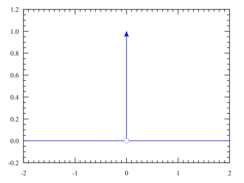
The Dirac delta \(\delta(x)\) is not a normal function, but a mathematical object (a distribution) that behaves like a probability density concentrated at a single point. It satisfies:
- \(\delta(x) = 0\) for all \(x \ne 0\)
- \(\int_{-\infty}^{\infty} \delta(x)\,dx = 1\)
More generally, a delta centered at a point \(a\) is written as \(\delta(x-a)\) and satisfies: $$ \int_{-\infty}^{\infty} \delta(x-a)\,dx = 1. $$
Important
The notation \(\delta(x-a)\) does not mean ordinary subtraction inside a normal function. It simply means a Dirac delta distribution centered at \(a\).
Intuitively, \(\delta(x-a)\) represents an "infinitely sharp spike" located exactly at \(x=a\), with total area \(1\). This is why it behaves like a tool that extracts the value of a function at \(a\): $$ \int_{-\infty}^{\infty} f(x)\,\delta(x-a)\,dx = f(a). $$
So \(\delta(x-a)\) is best understood as "a delta located at \(a\)".
Empirical
Suppose we have a dataset of \(m\) samples: $$ {x^{(1)}, x^{(2)}, \dots, x^{(m)}}. $$
Empirical distribution \(\hat{p}(x)\) is defined as: $$ \hat{p}(x) = \frac{1}{m} \sum_{i=1}^{m} \delta(x-x^{(i)}). $$
This means that the dataset assigns equal probability mass \(\frac{1}{m}\) to every observed sample.
Note
The empirical distribution in machine learning represents the distribution we actually train on. When we minimize training loss, we are minimizing an expectation under \(\hat{p}(x)\) rather than under the true unknown distribution \(p(x)\).
The empirical expectation of a function \(f(x)\) is:
So the standard dataset average used in deep learning is literally an expectation under the empirical distribution.
Note
The empirical distribution is a discrete approximation of the true data-generating distribution. Training a neural network is essentially an attempt to learn a model that generalizes beyond \(\hat{p}(x)\) and performs well on the true distribution \(p(x)\).
Mixture Distributions
Mixture distribution is a probability distribution formed by combining multiple simpler distributions. The idea is that the data may come from several different underlying sources, and each source has its own distribution. Suppose we have \(K\) component distributions: $$ p_1(x), p_2(x), \dots, p_K(x), $$ and mixture weights: $$ \pi_1,\pi_2,\dots,\pi_K, \qquad \pi_k \ge 0, \qquad \sum_{k=1}^K \pi_k = 1. $$
Then the mixture distribution is: $$ p(x) = \sum_{k=1}^K \pi_k p_k(x). $$
This can be interpreted as a two-step sampling process:
- First sample a component index: $ Z \sim \mathrm{Categorical}(\pi_1,\dots,\pi_K). $
- Then sample from the corresponding component distribution: $ X \sim p_Z(x). $
Note
The variable \(Z\) is called a latent variable because it is not directly observed, but it explains which component generated the data.
Note
Mixture models are widely used in probabilistic modeling because many real-world datasets are multi-modal. For example, the distribution of human heights in a population is not perfectly Gaussian, because it is better approximated as a mixture of two Gaussians (male and female). Similarly, pixel intensities in images often come from mixtures of different object materials, lighting conditions, and textures.
The most common mixture model is the Gaussian mixture model (GMM): $$ p(x) = \sum_{k=1}^K \pi_k \mathcal{N}(x;\mu_k,\Sigma_k). $$
Each component is a Gaussian with its own mean \(\mu_k\) and covariance matrix \(\Sigma_k\). GMMs are expressive enough to approximate many complex distributions, while still being mathematically tractable.
Note
Mixture models are a natural step toward deep generative models. Many modern models (including VAEs and diffusion models) can be viewed as learning complex mixtures in high-dimensional spaces.
Common Functions
Deep learning models often output unconstrained real numbers. However, many probabilistic parameters must satisfy constraints such as being in \((0,1)\) or summing to \(1\). For this reason, we use special nonlinear functions that map real-valued inputs into valid probability domains. The most common functions are described below.
Sigmoid
The logistic (sigmoid) function maps any real number to \((0,1)\): $$ \sigma(x) = \frac{1}{1+e^{-x}} = \frac{\exp(x)}{\exp(x)+\exp(0)}. $$
It is widely used to parameterize Bernoulli probabilities: $$ \phi = \sigma(z), \qquad Y \sim \mathrm{Bernoulli}(\phi). $$

Sigmoid is differentiable and also satisfies the symmetry identity: $$ 1-\sigma(x)=\sigma(-x). $$
Its inverse function is called the logit: $$ \forall x \in (0,1), \qquad \sigma^{-1}(x) = \log\Big(\frac{x}{1-x}\Big). $$
Important
Sigmoid saturates for large \(|x|\). When \(x \gg 0\), \(\sigma(x)\approx 1\), and when \(x \ll 0\), \(\sigma(x)\approx 0\). In both cases, the gradient \(\frac{d}{dx}\sigma(x)\) becomes close to \(0\), which slows down learning due to vanishing gradients. For this reason, sigmoid is rarely used as a hidden-layer activation in modern deep networks, and is usually replaced by ReLU or its variants.
Exercise
Find the derivative of the sigmoid function.
ReLU
Important
ReLU is not a probability concept. It does not parameterize a probability distribution and does not map values into a valid probability domain. It is primarily an activation function used in neural network architectures to improve optimization and gradient flow. We mention it here only because sigmoid saturation motivates why modern deep networks typically use ReLU-like activations in hidden layers.
The rectified linear unit (ReLU) is the most commonly used activation function in modern deep learning. It is defined as: $$ \mathrm{ReLU}(x)=\max(0,x). $$
ReLU is popular because it is simple, fast to compute, and avoids the strong saturation effect of sigmoid and tanh.

ReLU is piecewise linear, so its derivative is simple: $$ \frac{d}{dx}\mathrm{ReLU}(x) = \begin{cases} 0, & x < 0, \\ 1, & x > 0. \end{cases} $$
Note
ReLU is not differentiable at \(x=0\). However, researchers eventually realized that, this is not a practical issue in deep learning, because \(x=0\) occurs with probability nearly zero for continuous-valued activations. In implementations, the gradient at \(0\) is usually defined as \(0\) (a valid subgradient choice).
Important
ReLU has zero gradient for all negative inputs. If a neuron consistently outputs negative values, it may stop learning completely. This is called the dying ReLU problem. Variants such as Leaky ReLU and GELU are often used to reduce this effect.
Softplus
The softplus function maps \(\mathbb{R}\) to \((0,\infty)\): $$ \zeta(x) = \log(1+\exp(x)). $$
Note
Softplus is useful when a model parameter must be strictly positive (e.g variance \(\sigma^2 > 0\)).

Softplus is closely connected to sigmoid. In particular: $$ \log \sigma(x) = -\zeta(-x). $$
And its derivative is exactly sigmoid:
This is a useful fact in deep learning: softplus behaves like a smooth version of ReLU, but its gradient changes smoothly between \(0\) and \(1\). The inverse of softplus is: $$ \forall x>0, \qquad \zeta^{-1}(x)=\log(\exp(x)-1). $$
A useful symmetry identity is: $$ \zeta(x)-\zeta(-x)=x. $$
Note
In practice, we rarely implement softplus as \(\log(1+\exp(x))\) directly, because \(\exp(x)\) can overflow for large \(x\). Instead, deep learning libraries use numerically stable implementations.
Example
PyTorch provides:
torch.nn.functional.softplus(x)
Softplus is commonly used when a model must output a strictly positive parameter (such as a variance), since it guarantees positivity while still being smooth and differentiable.
Logarithm
Recall that the logarithm function \(\log(x)\) transforms products into sums. If we have independent samples, probabilities multiply: $$ P(x^{(1)},\dots,x^{(m)}) = \prod_{i=1}^m P(x^{(i)}). $$
Taking the logarithm converts this product into a sum: $$ \log P(x^{(1)},\dots,x^{(m)}) = \sum_{i=1}^m \log P(x^{(i)}). $$
This is the main reason why, say, maximum likelihood estimation is almost always performed using the log-likelihood instead of the raw likelihood.
Note
In machine learning, model parameters are often learned by maximum likelihood estimation (MLE). We choose parameters \(\theta\) that make the observed dataset most probable under the model. Suppose we have i.i.d. samples: $$ D={y^{(1)},\dots,y^{(m)}}. $$
The likelihood of the dataset is: $$ p(D \mid \theta) = \prod_{i=1}^{m} p!\big(y^{(i)} \mid \theta\big). $$
The MLE estimate \(\hat{\theta}_{\mathrm{MLE}}\) is defined as the value of \(\theta\) that maximizes this likelihood. In practice we maximize the log-likelihood instead: $$ \log p(D \mid \theta) = \sum_{i=1}^{m} \log p!\big(y^{(i)} \mid \theta\big). $$
Exercise
Suppose we observe \(m\) i.i.d. samples \(y^{(1)},\dots,y^{(m)}\) from a Bernoulli distribution with parameter \(\theta\). Write the likelihood function \(L(\theta \mid y^{(1)},\dots,y^{(m)})\) as a product. Then rewrite it as a log-likelihood (a sum).
The logarithm is only defined for \(x>0\). In particular: $$ \log(0) = -\infty $$
Note
This matters in deep learning because losses often contain \(\log(p)\) terms. If a model assigns probability \(p=0\) to the true outcome, the loss becomes infinite. In practice, this is handled by using numerically stable implementations (computing loss from logits) or by clamping probabilities with a small constant \(\epsilon>0\): $$ \log(p) \;\;\to\;\; \log(\max(p,\epsilon)). $$
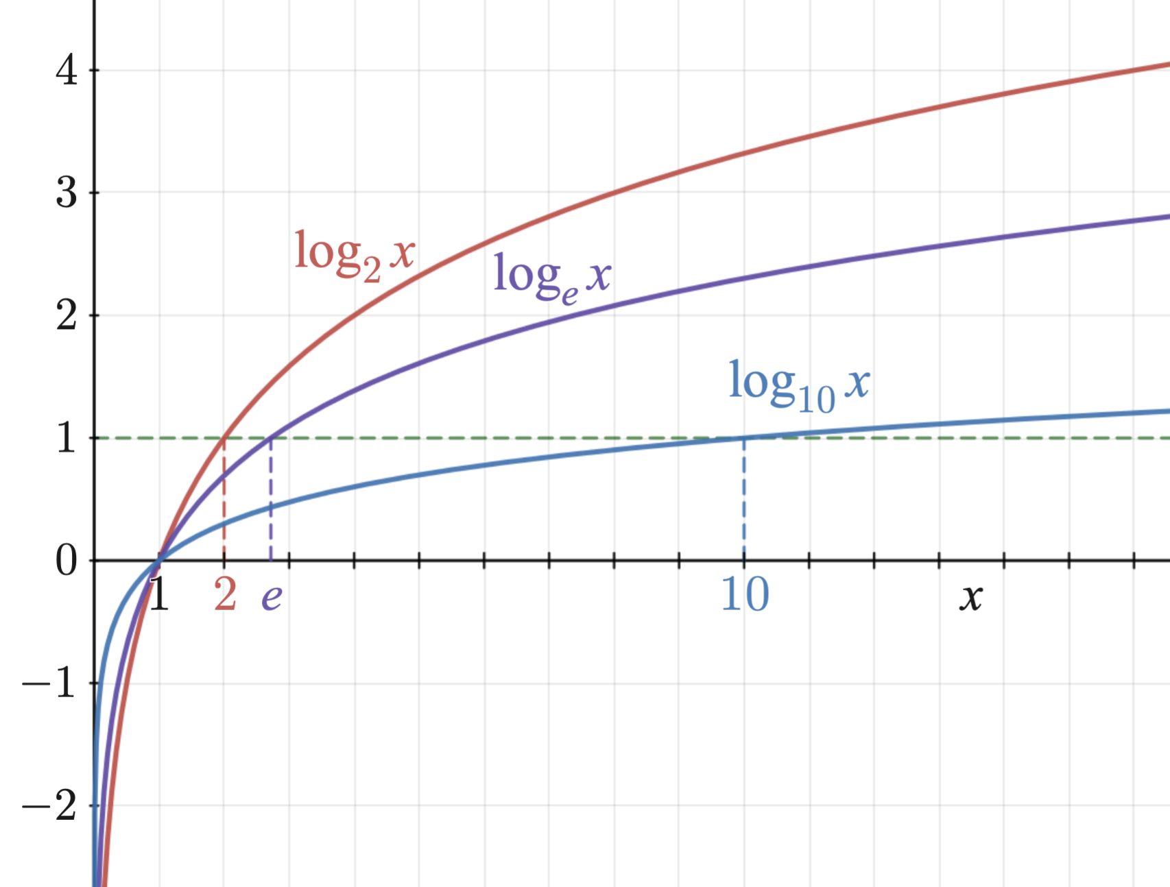
Logarithm is strictly increasing (monotonic): $$ x_1 < x_2 \quad\Rightarrow\quad \log(x_1) < \log(x_2). $$
Therefore, maximizing \(P(x)\) is equivalent to maximizing \(\log P(x)\): $$ \arg\max_x P(x) = \arg\max_x \log P(x). $$
Note
The derivative of log is \(\frac{1}{x}.\) This derivative becomes very large when \(x\) is close to \(0\), which is one reason why log strongly penalizes assigning very small probability to true outcomes.
Softmax
The softmax function maps logits \(z\in\mathbb{R}^k\) into a probability vector \(p\in\mathbb{R}^k\): $$ p = \mathrm{softmax}(z_i) = \frac{\exp(z_i)}{\sum_{j=1}^{k} \exp(z_j)}. $$
Softmax is also invariant to adding the same constant to all logits: $$ \mathrm{softmax}(z)=\mathrm{softmax}(z+c). $$
Important
For numerical stability, softmax is usually computed as: $$ \mathrm{softmax}(z) = \frac{\exp(z-\max(z))}{\sum_{j=1}^k \exp(z_j-\max(z))}. $$
Note
A logit is an unconstrained score in \((-\infty,\infty)\) that becomes a probability only after applying a transformation. For binary classification: $$ \phi=\sigma(z), \qquad z=\mathrm{logit}(\phi). $$ For multiclass classification: $\(p=\mathrm{softmax}(z).\)$
Working with logits is often preferred in deep learning because logits are numerically stable and easier to optimize than probabilities directly.
Measure Theory
When working with continuous probability distributions, some technical details require ideas from measure theory. In deep learning literature, we will encounter a few terms.
A set \(A\) is said to have measure zero if its total "size" is zero under integration. For example, a single point has measure zero. Any countable set of points also has measure zero. For example, the set of all rational numbers has measure zero, even though it is infinite.
A property is said to hold almost everywhere if it holds everywhere except on a measure-zero set. This means the property may fail on some special cases, but those cases occupy negligible space and do not affect integrals.
This terminology matters because many results that are always true in discrete probability only hold almost everywhere in the continuous case. In practice, these exceptions can usually be ignored.
Note
This is why deep learning often ignores edge cases. For example, ReLU is not differentiable at \(x=0\), but this does not matter in practice because the probability of hitting exactly \(x=0\) is almost zero for continuous-valued activations.
-
Kolmogorov, A.N. (1933, 1950). Foundations of the theory of probability. New York, US: Chelsea Publishing Company. ↩
-
A Dutch book argument says that if your probability assignments are inconsistent, someone can design a set of bets that guarantees you lose money no matter what happens. For example, if you assign \(P(A)=0.6\) and \(P(\neg A)=0.6\), then you are claiming both an event and its opposite are more likely than not. A bettor could sell you a bet on \(A\) and also sell you a bet on \(\neg A\), and you would overpay in total, while only one of them can ever pay out. This guarantees a loss. The probability axioms prevent such contradictions. ↩
-
A real coin is not infinitely thin, so in principle it could land on its edge. In practice this outcome is extremely rare, so it is usually ignored and the sample space is approximated as having only two outcomes. ↩
-
The term marginal is said to come from the traditional way of computing these sums on paper: one writes the joint distribution in a table and records the row and column totals in the margins of the page. ↩
-
The term multinoulli was popularized by Murphy (2012) as a playful name meaning "many Bernoullis." ↩
-
The distribution is called Gaussian because it was studied extensively by Carl Friedrich Gauss, especially in connection with measurement errors. ↩