The following material was initially prepared as a lecture for CSCI 4701: Deep Learning (Spring 2025) course at ADA University. The notebook is mainly based on Andrej Karpathy's lecture on Micrograd and is the continuation of my previous post called Python Code from Derivatives to Backpropagation.
![]()
Table of Contents
# This is a graph visualization code from micrograd, no need to understand the details
# https://github.com/karpathy/micrograd/blob/master/trace_graph.ipynb
from graphviz import Digraph

def trace(root):
    nodes, edges = set(), set()
    def build(v):
        if v not in nodes:
            nodes.add(v)
            for child in v._prev:
                edges.add((child, v))
                build(child)
    build(root)
    return nodes, edges

def draw_dot(root, format='svg', rankdir='LR'):
    """
    format: png | svg | ...
    rankdir: TB (top to bottom graph) | LR (left to right)
    """
    assert rankdir in ['LR', 'TB']
    nodes, edges = trace(root)
    dot = Digraph(format=format, graph_attr={'rankdir': rankdir}) #, node_attr={'rankdir': 'TB'})

    for n in nodes:
        dot.node(name=str(id(n)), label = "{ %s | data %.3f | grad %.3f }" % (n.label, n.data, n.grad), shape='record')
        if n._op:
            dot.node(name=str(id(n)) + n._op, label=n._op)
            dot.edge(str(id(n)) + n._op, str(id(n)))

    for n1, n2 in edges:
        dot.edge(str(id(n1)), str(id(n2)) + n2._op)

    return dot
Recall: Backpropagation
# This is the code from previous lecture
# It is important to understand _backward function
class Value:
  def __init__(self, data, _prev=(), _op='', label=''):
    self.data = data
    self._prev = _prev
    self._op = _op
    self.label = label
    self._backward = lambda: None
    self.grad = 0.0

  def __add__(self, other):
    data = self.data + other.data
    out = Value(data, (self, other),'+')

    def _backward():
      self.grad = 1.0 * out.grad
      other.grad = 1.0 * out.grad
    out._backward = _backward

    return out

  def __mul__(self, other):
    data = self.data * other.data
    out = Value(data, (self, other),'*')

    def _backward():
      self.grad = other.data * out.grad
      other.grad = self.data * out.grad
    out._backward = _backward

    return out

  def __sub__(self, other):
    return self + (Value(-1) * other) # self + (-other)

  def __repr__(self):
    return f'{self.label}: {self.data}'
a = Value(5, label='a')
b = Value(3, label='b')
c = a + b;   c.label = 'c'
d = Value(10, label='d')
L = c * d;   L.label = 'L'
draw_dot(L)

epochs = 10
learning_rate = 0.01

for _ in range(epochs):
  L.grad = 1.0

  # backward pass
  L._backward()
  c._backward()

  # optimization (gradient descent)
  a.data -= learning_rate * a.grad
  b.data -= learning_rate * b.grad
  d.data -= learning_rate * d.grad

  # forward pass
  c = a + b
  L = c * d

  print(f'Loss: {L.data:.2f}')
# output
Loss: 77.38
Loss: 74.81
Loss: 72.31
Loss: 69.87
Loss: 67.49
Loss: 65.16
Loss: 62.88
Loss: 60.66
Loss: 58.48
Loss: 56.35
# Equivalent implementation in PyTorch
# pay attention to requires_grad, no_grad() and zero_()

import torch

a = torch.tensor(5.0, requires_grad = True);
b = torch.tensor(3.0, requires_grad = True);
c = a + b
d = torch.tensor(10.0,requires_grad = True);
L = c * d

for _ in range(epochs):
  # backward pass
  L.backward()

  # optimization (gradient descent)
  with torch.no_grad():
    a -= learning_rate * a.grad
    b -= learning_rate * b.grad
    d -= learning_rate * d.grad

  # avoids accumulating gradients
  # comment this out to see how it affects the learning
  a.grad.zero_()
  b.grad.zero_()
  d.grad.zero_()

  # forward pass
  c = a + b
  L = c * d

  print(f'Loss: {L.data:.2f}')
# output
Loss: 77.38
Loss: 74.81
Loss: 72.31
Loss: 69.87
Loss: 67.49
Loss: 65.16
Loss: 62.88
Loss: 60.66
Loss: 58.48
Loss: 56.35
Activation Function
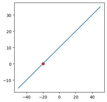
The function f(x) = x * w is a linear function always passing from origin. The real world data, however, will be much more complex, and in order to describe a pattern in the data our Machine Learning model should return a more flexible function. For that, we will do two things: add bias b and bring non-linearity with an activation function. We can choose different non-linear activation functions with the condition that it should be differentiable (otherwise we won’t be able to calculate gradients for backpropagation). We will implement sigmoid (logistic) activation function which has the following formula:

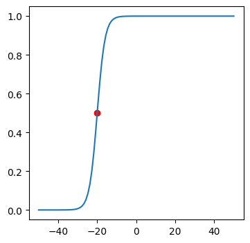
Sigmoid function not only makes a linear function non-linear and continuous, but also maps any value of x to be between 0 and 1. It may be useful when we want to predict probabilities for different output classes.
import numpy as np
import matplotlib.pyplot as plt
%matplotlib inline
def sigmoid(x):
  return 1.0 / (1 + np.exp(-x)) # see formula above
# a simple linear function where activation will be applied
def f(x, w=0.5, b=10, activation=None):
  out = x * w + b
  return activation(out) if activation else out
def plot(f, x, activation=None):
  plt.figure(figsize=(4, 4))
  x_all = np.linspace(-50, 50, 100)
  y_all = f(x_all, activation=activation)
  plt.plot(x_all, y_all)
  plt.scatter(x, f(x, activation=activation), color='r')
  plt.show()
x = -20
plot(f, x)
Now we will plot the exact same point mapped into the non-linear function between 0 and 1. Try out different x values and see the plots.
plot(f, x, sigmoid)
Exercise: Implement other activation functions (e.g. tanh, relu) and see the plot.
Exercise: What could be the distadvantage of using sigmoid activation function?
Artificial Neuron

An artificial neuron is simply a linear function passing through an activation function (e.g. sigmoid(x * w + b)). The illustration above describes an N-dimensional neuron, accepting inputs between x1 ... xn. The function f we had above is a very simple neuron with 1-dimensional input.
Question: What could be input values for predicting the probability of a customer cancelling their subscription?
Before creating our neuron, we will first make some updates to the Value class.
Not only Value class should have a sigmoid(x) function, but also it should be able to calculate a derivative for it.
Exercise: Find the derivative of the sigmoid function:
The requires_grad flag (similar to PyTorch) will tell which parameters are trainable and requires gradient calculation and update (Note that this feature is not implemented in micrograd).
For example, it doesn’t make sense to modify the real-life training inputs x1 and x2 for our neuron. We shouldn’t spend resources for calculating unnecessary gradients. Our goal is to nudge only the weight and bias (i.e. parameter) values, as well as the nodes dependent on them, in order to minimize the eventual loss.
class Value:
  def __init__(self, data, _prev=(), _op='', requires_grad=False, label=''):
    self.data = data
    self._prev = _prev
    self._op = _op
    self.label = label
    self._backward = lambda: None
    self.grad = 0.0
    self.requires_grad = requires_grad

  def __add__(self, other):
    data = self.data + other.data
    out = Value(data, (self, other), '+', self.requires_grad or other.requires_grad)

    def _backward():
      if self.requires_grad:
        self.grad = 1.0 * out.grad
      if other.requires_grad:
        other.grad = 1.0 * out.grad
    out._backward = _backward

    return out

  def __mul__(self, other):
    data = self.data * other.data
    out = Value(data, (self, other), '*', self.requires_grad or other.requires_grad)

    def _backward():
      if self.requires_grad:
        self.grad = other.data * out.grad
      if other.requires_grad:
        other.grad = self.data * out.grad
    out._backward = _backward

    return out

  def __sub__(self, other):
    return self + (Value(-1) * other) # self + (-other)

  def sigmoid(self):
    s = 1.0 / (1 + np.exp(-self.data))
    out = Value(s, (self, ), 'sigmoid', self.requires_grad)

    def _backward():
      if self.requires_grad:
        self.grad = s * (1.0 - s) * out.grad
    out._backward = _backward

    return out

  def __repr__(self):
    return f'Value({self.data:.4f})'
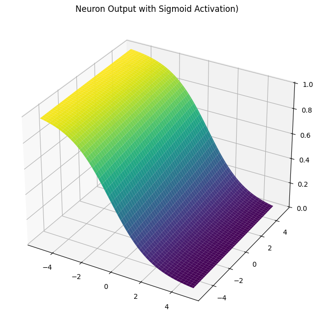
We will initially implement a simple Neuron class in 3D (2-dimensional input values and an output value). The function will have two inputs x1 and x2, which will become Value objects. Their weights w1 and w2 will determine how much input (e.g. age of a customer) influences outcome.
from mpl_toolkits.mplot3d import Axes3D

class Neuron:
  def __init__(self):
    self.w1 = Value(np.random.uniform(-1, 1), label='w1', requires_grad=True)
    self.w2 = Value(np.random.uniform(-1, 1), label='w2', requires_grad=True)
    self.b = Value(0, label='b', requires_grad=True)

  def __call__(self, x1, x2):
    out = x1 * self.w1 + x2 * self.w2 + self.b
    return out.sigmoid()

  # this code here is for plotting, no need to understand, works for only 3D
  def plot(self):
    x1_vals = np.linspace(-5, 5, 100)
    x2_vals = np.linspace(-5, 5, 100)
    X1, X2 = np.meshgrid(x1_vals, x2_vals)
    Z = np.zeros_like(X1)

    for i in range(X1.shape[0]):
      for j in range(X1.shape[1]):
        x1 = Value(X1[i, j])
        x2 = Value(X2[i, j])
        output = self(x1, x2)
        Z[i, j] = output.data

    fig = plt.figure(figsize=(10, 8))
    ax = fig.add_subplot(111, projection='3d')
    ax.plot_surface(X1, X2, Z, cmap='viridis')
    ax.set_title(f'Neuron Output with Sigmoid Activation)')
    plt.show()
Now we can initialize our inputs and neuron to see our computation graph. Our loss will be simple: the ground truth label y minus the predicted probability. Let’s assume that, our input values x1 and x2 correspond to a customer who made the purchase (y = 1). We will try out both activation functions and see their plots.
x1 = Value(2, label='x1')
x2 = Value(3, label='x2')
y  = Value(1, label= 'y')

n = Neuron()

pred = n(x1, x2);      pred.label = 'pred'
L = y - pred;          L.label = 'loss'
draw_dot(L)

n.plot()
The ground truth label 1 tells us that we should push our probability towards 1.0. In other words, as our loss L here is a simple error value corresponding to 1 - prob, we should try to minimize the loss down to zero with backpropagation. However, our computation graph is bigger than how it was before. The _backward pass function we call manually on each node is not scalable. Ideally, we should have a single function backward() to calculate all the gradients, which we previously saw in the PyTorch implementation. For that, we will need to sort the nodes of the computation graph (in this case, from input/weight nodes until the probability node). We can achieve that with a topological sort function implemented for micrograd.
topo = []
visited = set()
def build_topo(v):
  if v not in visited:
    visited.add(v)
    for child in v._prev:
      build_topo(child)
    topo.append(v)
build_topo(pred)
topo
We will integrate topological sort into our Value object and implement complete backward pass. We can also add a simple gradient descent function optimize() which will use this topology. Finally, instead of overriding gradients (=), we will accumulate them (+=) to avoid gradient update bugs when using the same node more than once in an operation. And as a consequence, we will have to reset gradients with zero_() (similar to PyTorch) so that the gradients of different backward passes will not affect each other (it does the exact same thing as self.grad = 0.0 was doing before gradient accumulation). Although, to be precise, zero_() function should reset only the gradient of self, and it is actually a function called zero_grad() of optimizer in PyTorch which resets gradients accross all nodes.
class Value:
  def __init__(self, data, _prev=(), _op='', requires_grad=False, label=''):
    self.data = data
    self._prev = _prev
    self._op = _op
    self.label = label
    self._backward = lambda: None
    self.grad = 0.0
    self.requires_grad = requires_grad
    self.topo = self.build_topo()
    self.params = [node for node in self.topo if node.requires_grad]

  def __add__(self, other):
    data = self.data + other.data
    out = Value(data, (self, other), '+', self.requires_grad or other.requires_grad)

    def _backward():
      if self.requires_grad:
        self.grad += 1.0 * out.grad
      if other.requires_grad:
        other.grad += 1.0 * out.grad
    out._backward = _backward

    return out

  def __mul__(self, other):
    data = self.data * other.data
    out = Value(data, (self, other), '*', self.requires_grad or other.requires_grad)

    def _backward():
      if self.requires_grad:
        self.grad += other.data * out.grad
      if other.requires_grad:
        other.grad += self.data * out.grad
    out._backward = _backward

    return out

  def __sub__(self, other):
    return self + (Value(-1) * other) # self + (-other)

  def sigmoid(self):
    s = 1.0 / (1 + np.exp(-self.data))
    out = Value(s, (self, ), 'sigmoid', self.requires_grad)

    def _backward():
      if self.requires_grad:
        self.grad += s * (1.0 - s) * out.grad
    out._backward = _backward

    return out

  def build_topo(self):
    # topological order all of the children in the graph
    topo = []
    visited = set()

    def _build_topo(node):
      if node not in visited:
        visited.add(node)
        for child in node._prev:
          _build_topo(child)
        topo.append(node)
    _build_topo(self)

    return topo

  def backward(self):
    if self.requires_grad:
      self.grad = 1.0
      for node in reversed(self.params):
        node._backward()

  def optimize(self, learning_rate=0.01):
    for node in self.params:
      node.data -= learning_rate * node.grad

  def zero_(self):
    self.grad = 0.0

  def zero_grad(self):
    for node in self.params:
      node.grad = 0.0

  def __repr__(self):
    return f'Value({self.data})'
In addition to the _backward() function which calculated the derivatives for only immediate previous nodes, we now have the backward() function which calculates derivates for all the nodes (we also won’t forget to set the gradient to 1.0 in the beginning). Once we plot the graph, pay attention that the input and leaf node gradients which we have no control over are not calculated, thanks to requires_grad.
x1 = Value(2, label='x1')
x2 = Value(5, label='x2')
y  = Value(1, label= 'y')

n = Neuron()

pred = n(x1, x2);      pred.label = 'pred'
L = y - pred;          L.label = 'loss'
L.backward()
draw_dot(L)

We can finally implement complete backpropogatation with the goal of increasing the final probability to 1.0 (decreasing the loss down to zero).
# gradient descent
L.optimize()

# forward pass
pred = n(x1, x2);      pred.label = 'pred'
L = y - pred;          L.label = 'loss'

draw_dot(L)

Let’s repeat the backpropagation in multiple epochs until we achieve a minimal loss. We will also print the parameters to see when our neuron function returns a maximum probability for the given input values. And we will make sure to not forget to reset the gradients.
while True:
  L.zero_grad()

  # backward pass
  L.backward()

  # gradient descent
  L.optimize()

  # forward pass
  pred = n(x1, x2);
  L = y - pred;

  print(f'Loss {L.data:.4f}')

  if L.data < 0.01:
    print(f'\nInputs: {x1} {x2}')
    print(f'Parameters: {n.w1} {n.w2} {n.b}')
    print(f'Prediction Probability: {pred.data}')
    break
# output
Loss 0.0148
Loss 0.0148
Loss 0.0147
...
Loss 0.0101
Loss 0.0100

Inputs: Value(2) Value(5)
Parameters: Value(0.15289672859342332) Value(0.8555124993367387) Value(0.013701999952082168)
Prediction Probability: 0.9900191690162561
N-dimensional Neuron
We have just now trained our 2-dimensional input neuron to find suitable parameter values for achieving a maximum probability for input values x1 and x2. Now we would like to create N-dimensional neuron which will accept much more inputs, similar to what we saw in the illustration of artificial neuron: x1 ... xn. As a consequence, our neuron will have to learn the parameter values for N-dimensional weights w1 ... wn.
class Neuron:
  def __init__(self, N):
    self.W = [Value(np.random.uniform(-1, 1), label=f'w{i}', requires_grad=True) for i in range(N)]
    self.b = Value(0, label='b', requires_grad=True)

  def __call__(self, X):
    out = sum((x * w for x, w in zip(X, self.W)), self.b)
    return out.sigmoid()
We will now see the training output of our N-dimensional neuron which will accept N Value inputs as a list. Note that our Neuron which implements sigmoid (logistic) activation is known as Logistic Regression.
X = [Value(x, label=f'x{i}') for i, x in enumerate([5, 0.4, -1, -2])]

n = Neuron(len(X))

pred = n(X);           pred.label = 'pred'
L = y - pred;          L.label = 'loss'
draw_dot(L)

while True:
  L.zero_grad()

  # backward pass
  L.backward()

  # gradient descent
  L.optimize()

  # forward pass
  pred = n(X)
  L = y - pred

  print(f'Loss {L.data:.4f}')

  if L.data < 0.01:
    print(f'\nInputs: {X}')
    print(f'Parameters: {n.W} {n.b}')
    print(f'Prediction Probability: {pred.data}')
    break
# output
Loss 0.1273
Loss 0.1235
Loss 0.1199
...
Loss 0.0101
Loss 0.0100

Inputs: [Value(5), Value(0.4), Value(-1), Value(-2)]
Parameters: [Value(0.6195076510193583), Value(0.988462556700058), Value(0.6814715991439656), Value(-0.8498024629867303)] Value(0.08692061974641961)
Prediction Probability: 0.9900282484345291
Artificial Neural Network

We managed to train our single neuron to learn a function for our input values. In reality, however, data is much more complex and we need to learn more complication functions. How to achieve that? By chaining many neurons together, similar to biological neuron. Each neuron will basically learn some portion of the overall function.
What we see above is an illustration of an artificial neural network. In the input layer we have three neurons, each separately accepting N-dimensional input values. The output values of each neuron are then fully connected, as inputs to the hidden layer with four neurons (note that there can be more than one hidden layer). And finally, the output of hidden layer neurons are passed as inputs to the output layer, which may, for example, predict probability scores for two classes.
We will now try to implement a fully connected feedforward neural network, which is often referred to as Multi-Layer Perceptron (MLP).
class Layer:
  def __init__(self, N, count):
    self.neurons = [Neuron(N) for _ in range(count)]

  def __call__(self, X):
    outs = [n(X) for n in self.neurons]
    return outs[0] if len(outs) == 1 else outs # flattening dimension if a single element
The code above creates a list of count number of neurons, each accepting N dimensional input. Let’s build our layers shown in the illustration above and connect them. Note that the input dimension of the next layer is the amount of neurons in the previous layer.
# input data and its dimension
X = [Value(x, label=f'x{i}') for i, x in enumerate([1, 4, -3, -2, 3])]
N = len(X)
# creating layers
in_layer = Layer(N, 3)
hid_layer = Layer(3, 4)
out_layer = Layer(4, 2)
# output of each layer is input to the next
X_hidden = in_layer(X)
X_output = hid_layer(X_hidden)
out = out_layer(X_output)
# let's plot either one of the outputs
draw_dot(out[0])

We will further abstract away the neuron and layer creation inside the MLP class. We will then reimplement the exact same network.
class MLP:
  def __init__(self, N, counts):
    dims = [N] + counts # concatenates dimensions
    self.layers = [Layer(dims[i], dims[i+1]) for i in range(len(dims)-1)]

  def __call__(self, X):
    out = X
    for layer in self.layers:
      out = layer(out)
    return out
nn = MLP(N, [3, 4, 2])
out = nn(X)
Iris Dataset
It is time to judge our network by applying it to the real dataset. Even though applying neural networks to Fisher’s Iris dataset is a little overkill (as the dataset is simple), it will be a nice demonstration of our MLP’s capacity.
Iris dataset has 4-dimensional input samples with three possible output classes. We should be able to predict the class of the Iris flower based on the width and height values of its two elements. We will load our dataset and split it into train and test sets.
from sklearn import datasets
from sklearn.model_selection import train_test_split

iris = datasets.load_iris()

X = iris.data  # 50x3 4-dimensional samples
y = iris.target # 3 classes (0, 1, 2)

X_train, X_test, y_train, y_test = train_test_split(X, y, test_size=0.2)

print(f'Train data shape: {X_train.shape}, {y_train.shape}')
print(f'Test data shape: {X_test.shape}, {y_test.shape}')
print(f'Input Samples:\n {X_train[:5]}')
print(f'Labels:\n {y_train[:5]}')
Train data shape: (120, 4), (120,)
Test data shape: (30, 4), (30,)
Input Samples:
 [[4.4 2.9 1.4 0.2]
 [4.7 3.2 1.3 0.2]
 [6.5 3.  5.5 1.8]
 [6.4 3.1 5.5 1.8]
 [6.3 2.5 5.  1.9]]
Labels:
 [0 0 2 2 2]
We should then convert each element to be a Value object. But before that, let’s try out two ready scikit-learn classifiers, LogisticRegression and MLPClassifier, the latter of which can be seen as the extension of the former, which we will implement in its simplistic form. As we have already discussed, LogisticRegression is basically our Neuron class which uses sigmoid (logistic) function as its activation. And in fact, Logistic Regression will simply be our MLP with the layer size for just a single neuron. Thanks to numpy vectorization and other optimizations, the sklearn implementations will be extremely quick.
from sklearn.linear_model import LogisticRegression
from sklearn.neural_network import MLPClassifier
from sklearn.metrics import accuracy_score

model = LogisticRegression()
model.fit(X_train, y_train)
preds = model.predict(X_test)
accuracy = accuracy_score(y_test, preds)
print(f"Logistic Regression Accuracy: {accuracy:.2f}")

model = MLPClassifier()
model.fit(X_train, y_train)
preds = model.predict(X_test)
accuracy = accuracy_score(y_test, preds)
print(f"MLP Classifier Accuracy: {accuracy:.2f}")
# output
Logistic Regression Accuracy: 1.00
MLP Classifier Accuracy: 1.00
When converting labels to Value objects, we can technically scale them down to be between 0 and 1 (by multiplying them to 0.5). Then we can apply the simple Mean Squared Error (MSE). Because there are only three labels and the dataset is small, it will work, yet it will penalize ordinal labels unnecessarily. For example, our loss should give the same penalty if we predict 0 instead of 1 or 2 (it is either one type of flower or another). MSE, however, will give more penalty when predicting 0 instead of 2 and less penalty when predicting 0 instead of 1 because of the imaginary distances between numbers, which do not exist among the real labels.
# converting numpy float arrays into Value lists
# scaling labels to be between 0 and 1 to simplify our code
# again, it is not a right way to treat the labels
X_train = [[Value(x) for x in X] for X in X_train]
X_test = [[Value(x) for x in X] for X in X_test]
y_train = [Value(y) * Value(0.5) for y in y_train]
y_test = [Value(y) * Value(0.5) for y in y_test]
Training Custom MLP Classifier
We will now create a class for our model, in the style of scikit-learn models, more specifically MLPClassifier.
As noted above, what we do is simple and will work in this case, but is not right. Ideally, we should initially one hot encode the ground truth labels to describe them with only zeros and ones. Our final layer for multiclass classification, instead of sigmoid activation, should output logits (unprocessed predictions) passing through softmax function. The loss in this case should be Categorical Cross Entropy instead of MSE.
Exercise (Advanced): Write code for the correct implementation noted above. See Josh Starmer’s (StatQuest) videos which explain its theory, including the Iris dataset, argmax and softmax functions, as well as Cross Entropy.
class Classifier:
  def __init__(self, layer_sizes=[2, 3, 1]):
    self.layer_sizes = layer_sizes
    self.nn = None
    self.L = None
    self.iterations = 0

  def forward(self, Xs):
    out = [self.nn(X) for X in Xs]
    return out

  def predict(self, X_test):
    return self.forward(X_test)

  def train(self, X_train, y_train, learning_rate=0.01):
    preds = self.forward(X_train)
    self.L = self.mean_squared_error(y_train, preds)
    self.L.zero_grad()
    self.L.backward()
    self.L.optimize(learning_rate=learning_rate)
    print(f'Loss: {self.L.data:.4f}')

  def fit(self, X_train, y_train, learning_rate=0.01, num_epochs=50):
    if not self.nn: # in order to not restart training if nn exists
      self.nn = MLP(len(X_train), self.layer_sizes)
    for i in range(num_epochs):
      print(f'Training epoch {self.iterations + i + 1}')
      self.train(X_train, y_train, learning_rate)
    self.iterations += i + 1

  def mean_squared_error(self, y_train, preds):
    return sum([(y-y_hat)*(y-y_hat) for y, y_hat in zip(y_train, preds)], Value(0))

  def score(self, y_test, preds):
    return self.mean_squared_error(y_test, preds).data / len(y_test)

  def accuracy_score(self, y_test, preds):
    # due to incorrect handling of the labels
    # we need to scale y_test and preds values back
    y_test = [y * Value(2) for y in y_test]
    preds = [y_hat * Value(2) for y_hat in preds]
    correct = sum(1 for y, y_hat in zip(y_test, preds) if round(y_hat.data) == y.data)
    total = len(y_test)
    return (correct/total)
Our naive classifer is ready and we can now train our model and note the accuracy. However, unlike the optimized classifiers of the sklearn library, it will be much slower and inefficient. Try out experiments with different layer sizes and learning rates, and notice how it affects the training process and loss. As we have mentioned before, we can implement Logistic Regression by simply passing layer_sizes=[1] to our MLP classifier.
model = Classifier([1])
# model = Classifier([4, 1])
model.fit(X_train, y_train, learning_rate=0.002, num_epochs=90)
# output
Training epoch 1
Loss: 54.7921
...

Loss: 1.3718
Training epoch 88
Loss: 1.3710
Training epoch 89
Loss: 1.3701
Training epoch 90
Loss: 1.3693
preds = model.predict(X_train)
print(f'Custom MLP classifier accuracy on train Data: {model.accuracy_score(y_train, preds):.2f}')
# output
Custom MLP classifier accuracy on train Data: 0.97
preds = model.predict(X_test)
print(f'Custom MLP classifier accuracy on test Data: {model.accuracy_score(y_test, preds):.2f}')
# output
Custom MLP classifier accuracy on test Data: 0.97
for i in range(10):
  print(y_test[i].data * 2, preds[i].data * 2)
# output
2.0 1.7378279677947062
1.0 1.3786491598121862
2.0 1.7797233124612888
2.0 1.5546211532302696
1.0 0.7808593322180695
1.0 1.1323777346177633
0.0 0.03179964376674919
2.0 1.6900839613983492
2.0 1.818651271834627
2.0 1.5712929781499119
2.0 1.9175600703929185