The following material was initially prepared as a lecture for CSCI 4701: Deep Learning (Spring 2025) course at ADA University. The notebook is mainly based on Andrej Karpathy's lecture on Micrograd.
![]()
Table of Contents
We will go from illustrating differentiation and finding derivatives in Python, all the way down till the implementation of the backpropagation algorithm.
Differentiation
import numpy as np
import matplotlib.pyplot as plt
%matplotlib inline
# simple x squared function
def f(x):
  return x**2
h = 1.0

dx = h
dy = f(x+h) - f(x)

print(f"Δx: {dx}")
print(f"Δy: {dy}")
print(f"When you change x by {dx} unit, y changes by {dy} units.")
# output
Δx: 1.0
Δy: 7.0
When you change x by 1.0 unit, y changes by 7.0 units.
def plot_delta(x, h, start=-4, stop=4, num=30):
  # np.linspace returns an array of num inputs within a range.
  x_all = np.linspace(start, stop, num)
  y_all = f(x_all)

  plt.figure(figsize=(4, 4))
  plt.plot(x_all, y_all)

  # dx & dy
  plt.plot([x, x + h], [f(x), f(x)], color='r')
  plt.plot([x + h, x + h], [f(x), f(x + h)], color='r')
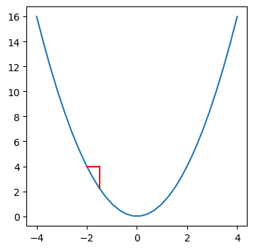
plot_delta(x=2, h=1)
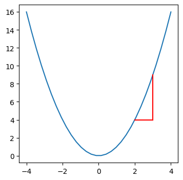
How to find if the ouput changes significantly when we change the input by some amount h?
def plot_roc(x, h):
  dx = h
  dy = f(x + h) - f(x)

  plot_delta(x, h)
  print(f"Rate of change is {dy / dx}")
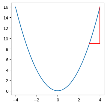
plot_roc(3, 1)
# output
Rate of change is 7.0
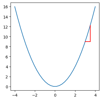
plot_roc(3, 0.5)
# output
Rate of change is 6.5
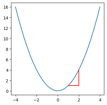
plot_roc(1, 1)
# output
Rate of change is 3.0
plot_roc(-2, 0.5)
# output
Rate of change is -3.5
The rate of change for different values of h are different at the same point x. We would like to come up with a single value that would tell how significantly y changes at a given point x within the function (a in the formula corresponds to x in the code).

Simply, this limit tells us how much the value of y will change when we change x by just a very small amount. Note: Essentially, derivative is a function.
x = 3
h = 0.000001 # limit of h approaches 0
d = (f(x + h) - f(x)) / h
print(f"The value of derivative function is {d}")
# output
The value of derivative function is 6.000001000927568
Partial Derivatives
Partial derivative with respect to some variable basically means how much the output will change when we nudge that variable by a very small amount.
Addition
f = lambda x, y: x + y
x = 2
y = 3
f(x, y) # 2+3=5
h = 0.000001
f(x + h, y)
# output
5.000001
Let’s see partial derivatives with respect to x an y.
# wrt x
(f(x + h, y) - f(x, y)) / h
# output
1.000000000139778
# wrt y
(f(x, y+h) - f(x, y)) / h
# output
1.000000000139778
It will always approach 1 for addition, no matter what are the input values.
for x, y in zip([-20, 2, 3], [300, 75, 10]):
  print(f'x={x}, y={y}: {(f(x + h, y) - f(x, y)) / h}')
x=-20, y=300: 0.9999999974752427
x=2, y=75: 0.9999999974752427
x=3, y=10: 1.0000000010279564
Indeed, if we have simple addition x + y, then increasing x or y by some amount will increase the result by the exact same amount. Assertion will work for any number h gets.
h = 10
assert f(x+h, y) - f(x, y) == h
assert f(x, y+h) - f(x, y) == h
Multiplication
f = lambda x, y: x * y
x = 2
y = 3
h = 1e-5 # same as 0.00001
(f(x + h, y) - f(x, y)) / h # wrt x
# output
3.000000000064062
for x in [-20, 2, 3]:
  print(f'x={x}, y={y}: {(f(x + h, y) - f(x, y)) / h}')
x=-20, y=3: 2.999999999531155
x=2, y=3: 3.000000000064062
x=3, y=3: 3.000000000064062
x = 10
h = 5
pdx = (f(x+h, y) - f(x, y)) / h
print(pdx, y)
assert round(pdx, 2) == round(y, 2)
# output
3.0 3
Complex
def f(a, b, c):
  return a**2 + b**3 - c
a = 2
b = 3
c = 4

f(a, b, c) #2^2+3^3-4=27
h = 1
f(a + h, b, c) #32
f(a + h, b, c) - f(a, b, c) #5
(f(a + h, b, c) - f(a, b, c)) / h #5
h = 0.00001 # when the change is approaching zero
pda = (f(a + h, b, c) - f(a, b, c)) / h
pda
# output
4.000010000027032
assert 2*a == round(pda)
Our function was f(a,b,c) = a2+b3-c. Partial derivative with respect to a is 2a (by the power rule), and when a=2 indeed we get 4.
Exercise: Code the partial derivative with respect to b and c and verify if the result correct.
Micrograd and Computation Graph
Based on Micrograd.
# Value class stores a number and "remembers" information about its origins
class Value:
  def __init__(self, data, _prev=(), _op='', label=''):
    self.data = data
    self._prev = _prev
    self._op = _op
    self.label = label
    self.grad = 0

  def __add__(self, other):
    data = self.data + other.data
    out = Value(data, (self, other), '+')
    return out

  def __mul__(self, other):
    data = self.data * other.data
    out = Value(data, (self, other), "*")
    return out

  def __repr__(self):
    return f"Value(data={self.data}, grad={self.grad})"
a = Value(5, label='a')
b = Value(3, label='b')
c = a + b; c.label = 'c'
d = Value(10, label='d')
L = c * d; L.label = 'L'
print(a, a._prev)
print(L, L._prev)
# output
Value(data=5, grad=0) ()
Value(data=80, grad=0) (Value(data=8, grad=0), Value(data=10, grad=0))
The computation graph of the function will be as follows:

Gradient
Gradient is vector of partial derivatives.
We want to know how much changing each variable will affect the output of L. We will store those partial derivatives inside each grad variable of each Value object.
L.grad = 1.0
The derivative of a variable with respect to itself is 1 (you get the same dx/dy).
f = lambda x: x
h = 1e-5
pdx = (f(x + h) - f(x)) / h
assert round(pdx) == 1
Now let’s see how changing other variables will affect the eventual result.
def f(ha=0, hb=0, hc=0, hd=0):
  # same function as before
  a = Value(5 + ha, label='a')
  b = Value(3 + hb, label='b')
  c = a + b + Value(hc); c.label = 'c'
  d = Value(10 + hd, label='d')
  L = c * d; L.label = 'L'
  return L.data
h = 1e-5
(f(hd=h) - f()) / h
# output
7.999999999697137
From the computational graph we can also see that L=c*d. When we change the value of d just a little bit (derivative of L with respect to d) the value of L will change by the amount of c, which is 8.0. We saw it above in the partial derivative of a multiplication.
d.grad = c.data
c.grad = d.data
With the same logic, the derivative of L wrt c will be the value of d, which is 10.0. We can verify it.
(f(hc=h) - f()) / h
#output
10.000000000331966
Chain Rule
To determine how much changing earlier variables in the computation graph will affect the L variable, we can apply the chain rule. Simply, the derivative of L with respect to a is the derivative of c with respect to a multiplied by the derivative of L with respect to c. God bless Leibniz.

The derivate of c both wrt a and ‘b’ is 1 due to the property of addition shown before (c=a+b). From here:
a.grad = 1.0 * c.grad
b.grad = 1.0 * c.grad

a.grad, b.grad
# output
(10.0, 10.0)
We can verify it as well. Let’s see how much L gets affected, when we shift a or b by a small amount.
(f(ha=h) - f()) / h
# output
10.000000000331966
(f(hb=h) - f()) / h
# output
10.000000000331966
We will finally redraw the manually updated computation graph.

It basically implies that, for example, changing the value of a by 1 unit (from 5 to 6) will increase the value of L by 10 units (from 80 to 90).
f(ha=1)
# output
90
f(hb=1), f(hc=1), f(hd=1) # the rest of the cases
# output
(90, 90, 88)
Optimization with Gradient Descent
What we saw above was one backward pass done manually. We are mainly interested in the signs of partial derivatives to know if they are positively or negatively influencing the eventual loss L of our model. In our case, all the derivatives are positive and influence loss positively.
We have to simply nudge the values in the opposite direction of the gradient to bring the loss down. This is known as gradient descent.
lr = 0.01 # we will discuss learning rate later on

a.data -= lr * a.grad
b.data -= lr * b.grad
d.data -= lr * d.grad

# we skip c which is controlled by the values of a and b
# pay attention that the rest are leaf nodes in the computation graph
In case the loss is a negative value (not common), we will need to “gradient ascend” the loss upwards towards zero and change the sign to += from -=. Note that the values of parameters (a, b, d) can decrease or increase depending on the sign of grad.
Forward Pass
We will now do a single forward pass to see if loss has been decreased. Previous loss was 80.
# We will now forward pass
c = a + b
L = c * d

L.data
# output
77.376
We optimized our values and brought down the loss.
Backward Pass
Manually calculating gradient is good only for educational purposes. We should implement automatic backward pass which will calculate gradients. We will rewrite our Value class for backward pass.
class Value:
  def __init__(self, data, _prev=(), _op='', label=''):
    self.data = data
    self._prev = _prev
    self._op = _op
    self.label = label
    self.grad = 0.0
    self._backward = lambda: None # initially it is a function which does nothing

  def __add__(self, other):
    data = self.data + other.data
    out = Value(data, (self, other), '+')

    def _backward():
      self.grad = 1.0 * out.grad
      other.grad = 1.0 * out.grad
    out._backward = _backward

    return out

  def __mul__(self, other):
    data = self.data * other.data
    out = Value(data, (self, other), "*")

    def _backward():
      self.grad = other.data * out.grad
      other.grad = self.data * out.grad
    out._backward = _backward

    return out

  def __repr__(self):
    return f"Value(data={self.data}, grad={self.grad})"
# Recreating the same function
a = Value(5, label='a')
b = Value(3, label='b')
c = a + b; c.label = 'c'
d = Value(10, label='d')
L = c * d; L.label = 'L'

We will initialize the gradient of the loss to be 1.0 and then call backward() function. We should get the same results which we manually calculated previously.
L.grad = 1.0
L._backward()
c._backward()

Exercise: Make sure that all operations and their partial derivatives can be calculated (e.g. division, power).
Training Model with Backpropagation
We can now call the optimization process, as well as forward and backward passes to reduce loss. Training model with the help of backward pass, optimization, and forward pass is called backpropagation.
# optimization
lr = 0.01
a.data -= lr * a.grad
b.data -= lr * b.grad
d.data -= lr * d.grad

# forward pass
c = a + b
L = c * d

# backward pass
L.grad = 1.0
L._backward()
c._backward()

L.data # loss
# output
74.8149472
We have now trained the model for a single epoch. Even though what we do is oversimplistic and not precise, the main intuition and concepts behind training a neural network is the same.
We will train the model for multiple epochs until we reduce the loss down to zero.
while True:
  # optimization
  a.data -= lr * a.grad
  b.data -= lr * b.grad
  d.data -= lr * d.grad

  # forward pass
  c = a + b
  L = c * d

  # backward pass
  L.grad = 1.0
  L._backward()
  c._backward()

  if L.data < 0:
    break

  print(f'Loss: {L.data}')
# output
Loss: 72.31
Loss: 69.87
Loss: 67.49
...
...
Loss: 1.8
Loss: 0.45
PyTorch Implementation
All we did manually is built in to PyTorch. We will do a forward and backward pass and check if the gradients are what we had previosuly calculated. As gradients are not always calculated, for optimization purposes requires_grad is set to False by default. We cannot also calculate gradient for leaf nodes.
import torch

a = torch.tensor(5.0);    a.requires_grad = True
b = torch.tensor(3.0);    b.requires_grad = True
c = a + b
d = torch.tensor(10.0);   d.requires_grad = True
L = c * d
L.backward()
a.grad, b.grad, d.grad
# output
(tensor(10.), tensor(10.), tensor(8.))
We got the expected result.