This article introduces the emerging and popular area in Artificial Intelligence called Deep Learning and is based on Chapter 1 of the famous Deep Learning book by Ian Goodfellow, Yoshua Bengio, and Aaron Courville. The book was written in 2016 and can be considered to be old by today’s rapid technological advancement standards. However, as far as I know, it is the book that extensively explores deep learning at the highest quality, and is freely available online as well.
Andrew Ng’s well-known courses on Deep Learning Specialization were indeed a great introduction to deep learning. However, my current aim is to have my time and slowly study deep learning in greater detail. Of course, I (which means also you) should always keep in mind that some concepts/claims mentioned in the book naturally became outdated in the past 6 years. But it should not affect our experience much, as the core principles guiding deep learning remain the same over the years.
Keywords
In addition to Table of Contents, I decided to include keywords, referring to important concepts in the article. You can CTRL/CMD + F the keywords and find them in the article to read:
knowledge base approach, machine learning, representation learning, factors of variation, defining deep learning, evolution of deep learning, three waves of development, cybernetics, connectionism, artificial neural networks, linear models, distributed representation, MNIST, data size, model size
Table of Contents
Introduction
The challenging part of Artificial Intelligence (AI) is solving tasks that humans perform intuitively but have a hard time describing how it is done. 1 Like face recognition. We will concentrate on this issue by building systems gradually and allowing machines to learn from experience. As every concept is built upon simpler concepts, with many layers, it got the name of Deep Learning. In this case, there is no need for a programmer to formally define rules for AI to perform.
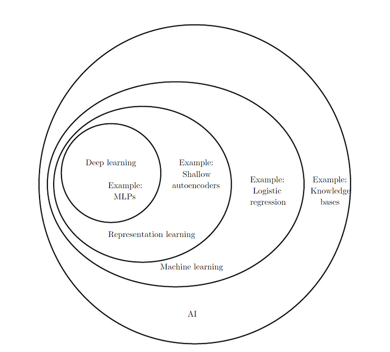
The knowledge Base approach to AI is hard-coding rules about the problem environment in formal languages. This approach never had a major success (for example, Cyc).
Machine Learning (ML), on the other hand, is the capability of an Artificial Intelligence program to extract its own knowledge from data patterns. With the help of ML, it is possible to tackle problems that may have subjective solutions. For example, a simple ML algorithm, logistic regression, can recommend Cesarian delivery (Mor-Yosef et al. 1990), and naïve Bayes can filter out spam emails.
Representation Learning
Algorithms depend on the data representation. For example, if a doctor will not define information — features about the MRI of a patient (e.g. existence of an unusual element in the scan), then logistic regression will not be able to come up with its own features and predict the outcome. Therefore, careful and precise choice of representation can drastically increase the algorithm performance (e.g. using Arabic instead of Roman numbers for arithmetic operations).
The choice of a correct set of features will guide an ML algorithm and help to increase its performance. But it is not always intuitive for a human to understand which features exactly need to be extracted. Hence, it makes sense to have an algorithm that will learn the representations on its own as well. Naturally, we call this representation learning, which is a much faster and more reliable way of defining features. Autoencoder, which will be discussed later in the chapters, is a fine example of representation learning.
Factors of variation
When reading the book, it was complicated to understand the paragraph explaining the term factors of variation. Luckily, I was not the only one, and the question had been posted on StackExchange, when user OmG had the following definition:
“Factors of variation are some factors which determine varieties in observed data. If that factors change, the behavior of the data will change. […] these factors are usually independent and one factor does not change by changing the value of the others.”
For example, factors of variation in a car image might be the car’s color, position, the brightness of the sun, etc. But the problem is that these factors of variation might have some effect on each data image (e.g. the car’s bright pixel color may become dark at night). We need to disentangle the factors of variation and get rid of those that we find to be unnecessary.
At times, it is quite challenging to automatically extract certain features (e.g. accent of a speaker) from data. In deep learning, it is tackled by having simpler representations representing representations.
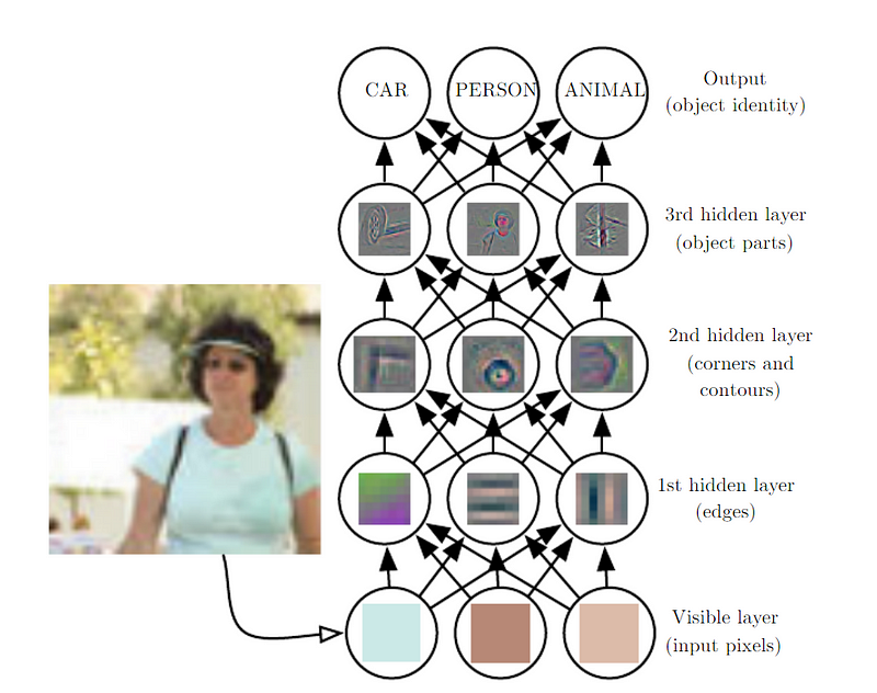
Multilayer Perceptron (MLP) is simply a mathematical function mapping input to output. Simpler functions generate more complicated functions, and as a result of different functions, we get different representations.
Deep learning’s goal is to find the right representation. We can think of each representation layer as a memory state with parallelly executed instructions. Not necessarily every activation stores factors of variation; some activations may encode information about the state of the program. Just like counter or pointer.
Defining Deep Learning
The book summarizes the concept of deep learning in the following manner:
“[Deep learning] is a type of machine learning, a technique that enables computer systems to improve with experience and data. […] [It] achieves great power and flexibility by representing the world as a nested hierarchy of concepts, with each concept defined in relation to simpler concepts, and more abstract representations computed in terms of less abstract ones.”
Note: Depth of a deep learning model can be measured in two ways: 1) depth of the computational graph, 2) depth of the probabilistic modeling graph. But as the longest path from the input of the model to its output is often subjective, and as there is no consensus in understanding which measurement is more relevant, we can shuffle off these terms (although you may refer to pages 7 and 8 of the book for the explanation). The only thing that we need to know is that deep learning models are composed of a greater number of functions/concepts than the traditional ML.
Evolution of Deep Learning
Deep learning is not a new research area, it just became popular only recently due to the increase in the available data and computational power (more about them later). There have been three waves of development in deep learning: 1) cybernetics (1940s–60s), 2) connectionism (1980s-90s), and 3) deep learning (2016-ongoing).
THE FIRST WAVE
Cybernetics, inspired by the biological learning theories (McCulloch & Pitts 1943, Hebb 1949) introduced the first models (perceptron) to train a single neuron (Rosenblatt 1958). Connectionism introduced backpropagation (Rumelhart et al. 1986a) and trained a neural network with hidden layer. Contemporary Deep Learning emerged around 2006 (Hinton et al. 2006, Bengio et al. 2007, Ranzato et al. 2007a).
As in its initial form, deep learning concepts were inspired by biological theories, i.e. from biological neurons (McCulloch-Pitts neuron), it was often referred to as Artificial Neural Networks (ANN). However, deep learning is not the exact modeling of real neural networks located in the biological brain.
Linear models are models making use of the linear function used by perceptron and Adaptive linear element (ADALINE — Widrow & Hoff 1960). 2 A crucial limitation of linear functions is that they cannot learn the XOR function, which reduced the popularity of deep learning during the 1970s.
As we don’t know exactly how the brain works, we cannot correctly imitate it while creating our artificial neural networks. Yet, we can get inspired by neuroscience and extract certain ideas from it. Neocognitron (Fukushima 1980), the predecessor of Convolutional Neural Networks (CNN — LeCun et al 1998b), for example, was based on the visual system of mammals. Certain network architectures were also inspired by neuroscience.
However, the authors of the book claim that we should not approach modern deep learning with the purpose of simulating the brain, as neural networks combine knowledge from different areas, including but not bound to, linear algebra, probability, numeric optimization, and information theory. Exploring the algorithmic behavior of the brain is called computational neuroscience which is an interesting and also a separate scientific sphere.
THE SECOND WAVE
With the emergence of parallel distributed processing, also known as connectionism, which was based on cognitive science, the second wave of deep learning started to develop. The idea was that, when networked together, lots of simple computational units could act intelligently.
Distributed representation (Hinton et al 1986) implies that many features should represent each input when each feature should also represent many inputs. A simple example arises when we want to create a model that has to detect three objects — A, B, C, and their three colors — red, green, blue. We can have 9 possible combinations to reach the solution with their neuron activations (e.g. red_A, red_B, red_C, green_A, etc). Or, which is more efficient, we can use distributed representation. That is, we can have only 6 neurons: 3 neurons for identifying the color, and 3 neurons for defining the object. In this case, each color can be learned from the images of all three objects instead of only one. Chapter 15 of the book describes the distributed representation in greater detail.
The backpropagation algorithm was also the result of the second wave of deep learning during the 1980s. Long short-term memory (LSTM — Hochreiter & Schmidhuber 1997) was implemented to resolve the mathematical difficulties that arose from modeling long sequences.
Nevertheless, deep learning was still losing the competition against other machine learning algorithms, and therefore its popularity was decreasing since the mid-1990s. Luckily, The Canadian Institute for Advanced Research (CIFAR) invested in its Neural Computation and Adaptive Perception (NCAP) project, uniting different influential ML research groups, and continued the research on neural networks.
THE THIRD WAVE
Finally, in 2006, Geoffrey Hinton, whose name you will hear often, made a breakthrough with the deep belief network trained by the layer-wise pretraining strategy (Hinton et al. 2006). It soon became clear that other networks could also implement the same strategy in order to achieve efficiency and even outperform other ML systems.
Data Size
It is crucial that now we don’t lack resources for deep learning algorithms to train. Data has increased drastically over time due to the digitization of our society, when it is easy to automatically record the actions of people who interact with computers. That gave rise to the age of “Big Data”.
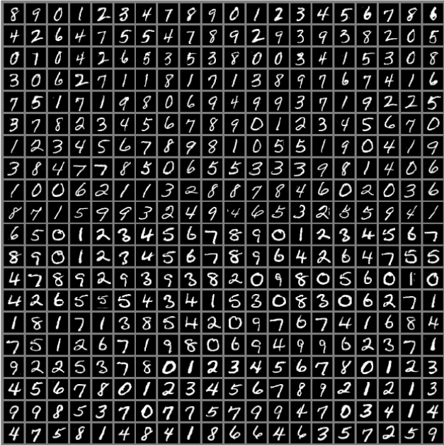
The most famous machine learning database MNIST was collected by the National Institute of Standards and Technology (NIST), and later was modified (hence the M before NIST) for simpler usage of ML algorithms. Geoffrey Hinton called this dataset “the drosophila of ML”. For those who don’t know it (quickly googles), drosophila is a fruit fly extensively used in genetic research labs.
An interesting rule of thumb is mentioned in the book about the performance of neural networks based on data size:
“As of 2016, a rough rule of thumb is that a supervised deep learning algorithm will generally achieve acceptable performance with around 5,000 labeled examples per category and will match or exceed human performance when trained with a dataset containing at least 10 million labeled examples.”
It is a current research area to work with smaller datasets while dealing with large unlabeled data with unsupervised/semi-supervised learning.
Model Size
In addition to the increased data size, we also now have the computational power to train bigger networks. The neural networks used to be very small back in the day and naturally didn’t accomplish much. It’s worth noting that even today’s largest artificial neural networks are smaller than the nervous system of a frog. However, the computational power (CPU, GPU, TPU) will continue to increase over time, and hopefully, we will be able to implement the same number of artificial neurons as the real neurons in the human brain by the year of 2050.
Increased Impact of Deep Learning
ImageNet Large Scale Visual Recognition Challenge (ILSVRC) is the biggest object detection competition and is held yearly. It was a sensation when a convolutional neural network won the contest by a large margin (Krizhevsky et al 2012). Speech recognition and image segmentation are also the areas where deep learning has a lasting impact.
Over time, more complex problems are being tackled with deep learning. The book was written in 2016, and naturally, the recent revolutions in the area of deep learning aren’t mentioned in this chapter. However, it is worth noting that the sequence learning with LSTMs had a huge impact on machine translation, when the emergence of neural Turing machines (Graves et al 2014) allowed to read and modify the memory cells, re-introducing the concept of self-programming.
The book mentions the advances in reinforcement learning with DeepMind’s Atari project, naturally “forgetting” about the revolutionary AlphaZero — the research published a year after the book (Silver et al 2017). Finally, deep learning influenced other fields as well, when an example is predicting molecule interactions in order to design new drugs.
Footnotes
-
If we can articulate the thinking process, then AI will have no fuss with solving a problem, even if it is mentally challenging for a human to tackle it. Like playing the game of Chess. ↩
-
I suppose that many concepts will be discussed later on in the book, in which case, I will elaborate on them in future articles. Otherwise, I will return back and update this article and explain ADALINE and other possible unclear terms so far. ↩